Probability & Statistics
At a glance
You need this in: Week 02 (splitting), Week 04 (metrics), Week 09 (model selection), and all of Project 2 Estimated time: 35 minutes Assumed: you know what a mean, a histogram, and a percentage are
Probability is a vast subject and almost all of it is irrelevant here. This page covers the four things the course asks of you that genuinely require it: understanding what a random split assumes, reading precision and recall correctly, handling a skewed target, and saying whether one model is really better than another.
The last one is the payoff. Project 2 asks for an explicit claim about which differences between models are real, and section 8 is how you make one.
1. A column is a sample from a distribution
The prices in your dataset are not the prices. They are a sample from all the listings that exist, or will exist. A model is only useful because it learns something about that larger population, and every question about evaluation is really a question about how well a sample stands in for it.
Hold that thought. Almost everything below follows from it.
2. Three shapes you will meet
Bernoulli. A yes or no outcome with probability \(p\) of yes. Every binary target is one. The class balance of your dataset is your estimate of \(p\).
Normal. The symmetric bell curve, described completely by its mean and standard deviation. The residuals of a good regression look roughly like this, and it is the default assumption behind a lot of statistics.
Right-skewed. Most values modest, a few very large. Prices, salaries, and counts almost always look like this, and it matters more than the other two put together.
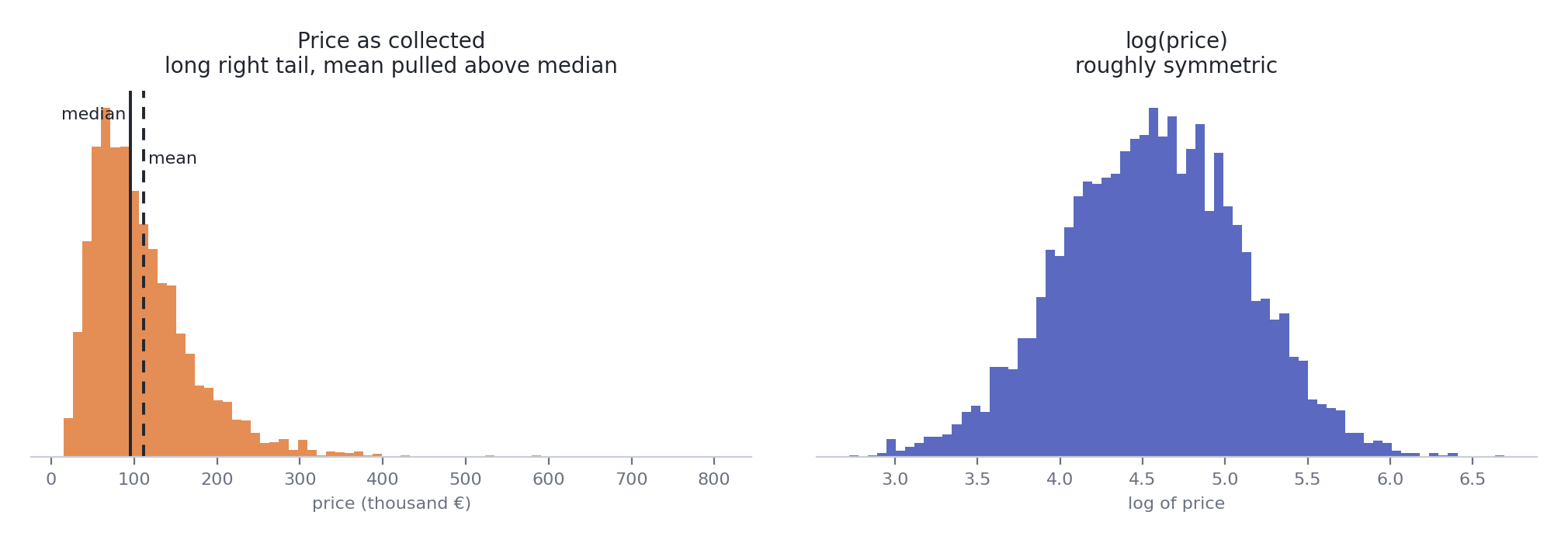
Synthetic apartment prices. The long tail drags the mean above the median. Taking the log pulls the tail in and makes the distribution roughly symmetric.
A skewed target causes two problems. The few expensive listings dominate the squared error, so the model spends its effort on them. And the errors grow with the price, so a single error measure hides very different performance at the cheap and expensive ends.
The usual fix is to model the log and convert back:
y_log = np.log1p(y_train)            # log(1 + y), safe at zero
model.fit(X_train, y_log)
y_pred = np.expm1(model.predict(X_test))
Where this lands
Week 3, as a feature engineering decision, and it will matter for the course dataset. One consequence worth knowing: an error in log space is roughly a percentage error in the original units. That is often closer to what people care about, since being 20,000 euros out on a 60,000 flat is far worse than on a 600,000 villa.
3. Expectation and variance
The expectation \(E[X]\) is the long-run average. The variance \(\text{Var}[X]\) measures spread, and the standard deviation is its square root, in the same units as the data.
One fact carries more of this course than any other:
The average of \(n\) independent measurements is less noisy than any single one, and the noise shrinks with the square root of \(n\). Two consequences:
- A score averaged over five cross-validation folds is more trustworthy than a score from one split.
- A test set of 50 rows gives a noisy score. Quadrupling it only halves the noise.
4. What a random split assumes
A random train and test split quietly assumes the rows are i.i.d.: independent and identically distributed.
Independent means one row tells you nothing about another. Identically distributed means the test rows, and the future rows the model will face, come from the same distribution as the training rows.
When either breaks, a random split lies to you, and it lies in your favour.
| Situation | What breaks | What to do instead |
|---|---|---|
| The same building is listed several times | Independence. Copies land on both sides of the split and the model effectively sees the test set. | Grouped split, keeping every listing from one building together |
| Data collected over time | Identical distribution. The future differs from the past, and neighbouring days resemble each other. | Temporal split, training on the past and testing on the later period |
| A rare class | Nothing breaks, but a random split can leave the test set with almost none of it | Stratified split |
Where this lands
Week 2. Choosing the split is choosing which assumption you are willing to make about your data. This table is the whole lesson in compressed form.
5. Precision and recall are conditional probabilities
\(P(A \mid B)\) is the probability of \(A\) given that \(B\) happened.
With \(y\) the truth and \(\hat{y}\) the prediction:
Precision: of the cases I flagged, how many were real? Recall: of the real cases, how many did I flag?
Same numerator, the true positives. Different denominators, pointing in opposite directions. Once you see them as two conditional probabilities looking at the same table from different sides, you stop confusing them.
| Predicted positive | Predicted negative | |
|---|---|---|
| Actually positive | true positive | false negative |
| Actually negative | false positive | true negative |
Precision reads down the first column. Recall reads along the first row.
6. Base rates, and why accuracy lies
A condition affects 1% of 10,000 people, so 100 have it. A test catches 99% of real cases and wrongly flags 1% of healthy people.
- True positives: 99 of the 100
- False positives: 1% of 9,900, which is 99
- Precision: 99 / (99 + 99) = 50%
A test that sounds 99% reliable is right only half the time it says yes, because the healthy group is so much larger that even a small error rate on it swamps the real cases.
It gets worse. A "model" that says no to everyone scores 99% accuracy and catches nobody.
Where this lands
Week 4. Whenever one class is rare, accuracy is close to meaningless. Look at precision and recall, and at the precision-recall curve rather than the ROC curve. The metrics page goes into which to choose.
7. Your test score is a random variable
Split the data differently and you get a different score. Same model, same data, different number.
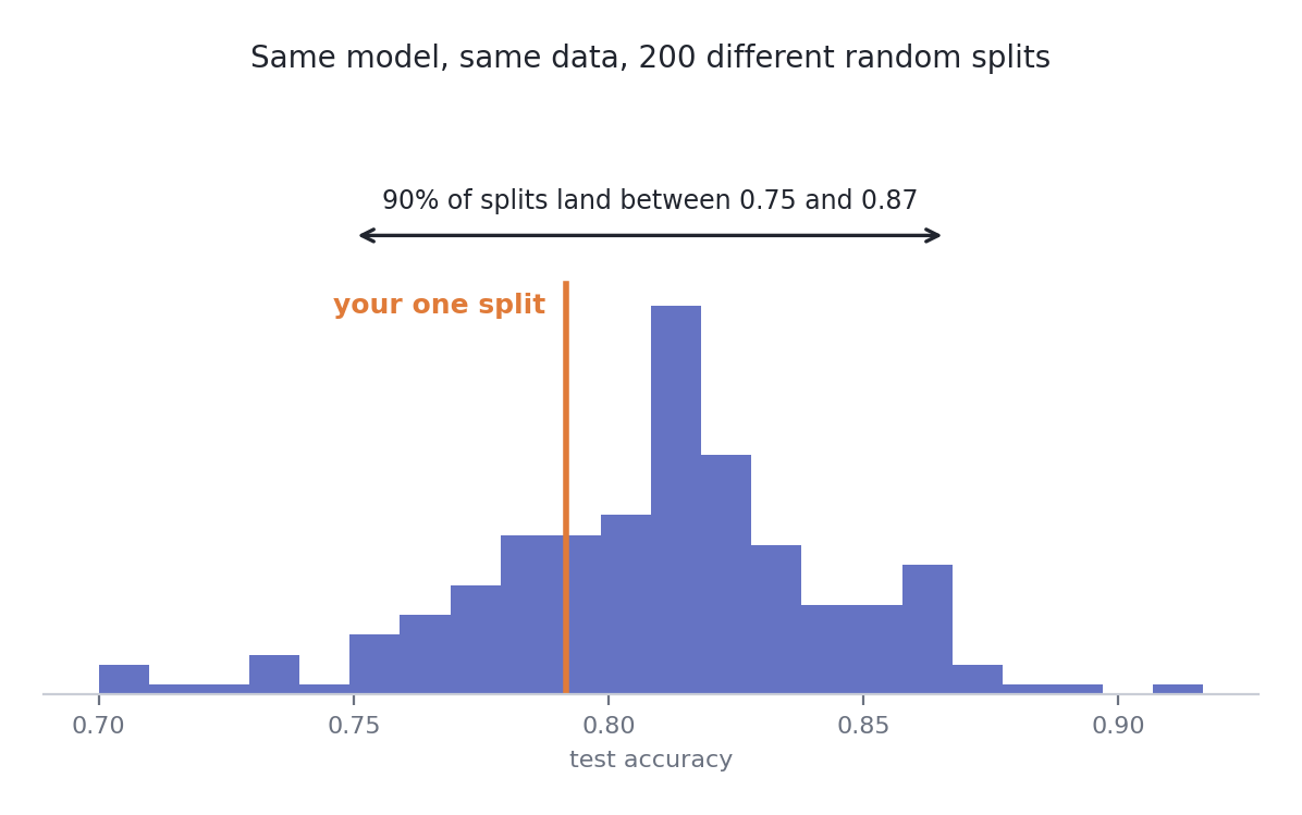
One logistic regression, one synthetic dataset, 200 random splits. The score you report depends heavily on which split you happened to draw.
Your single test score is one draw from that histogram. A one-point improvement measured on one split can be entirely luck of the draw. This is the reason cross-validation exists, and the reason every score in your projects comes with a spread attached.
8. Is the difference real?
The practical method, in three parts.
Report a spread, never a single number. Mean and standard deviation across folds.
Compare on the same folds. Some folds are simply harder than others, and a hard fold drags both models down together. Comparing fold by fold cancels that shared difficulty out, which is far more sensitive than comparing two averages.
Count the wins. If model B beats model A on nearly every fold, that is a claim. If it wins on about half, it is noise.
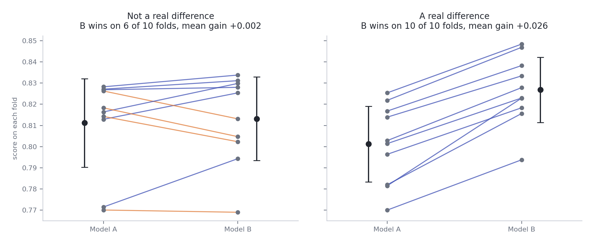
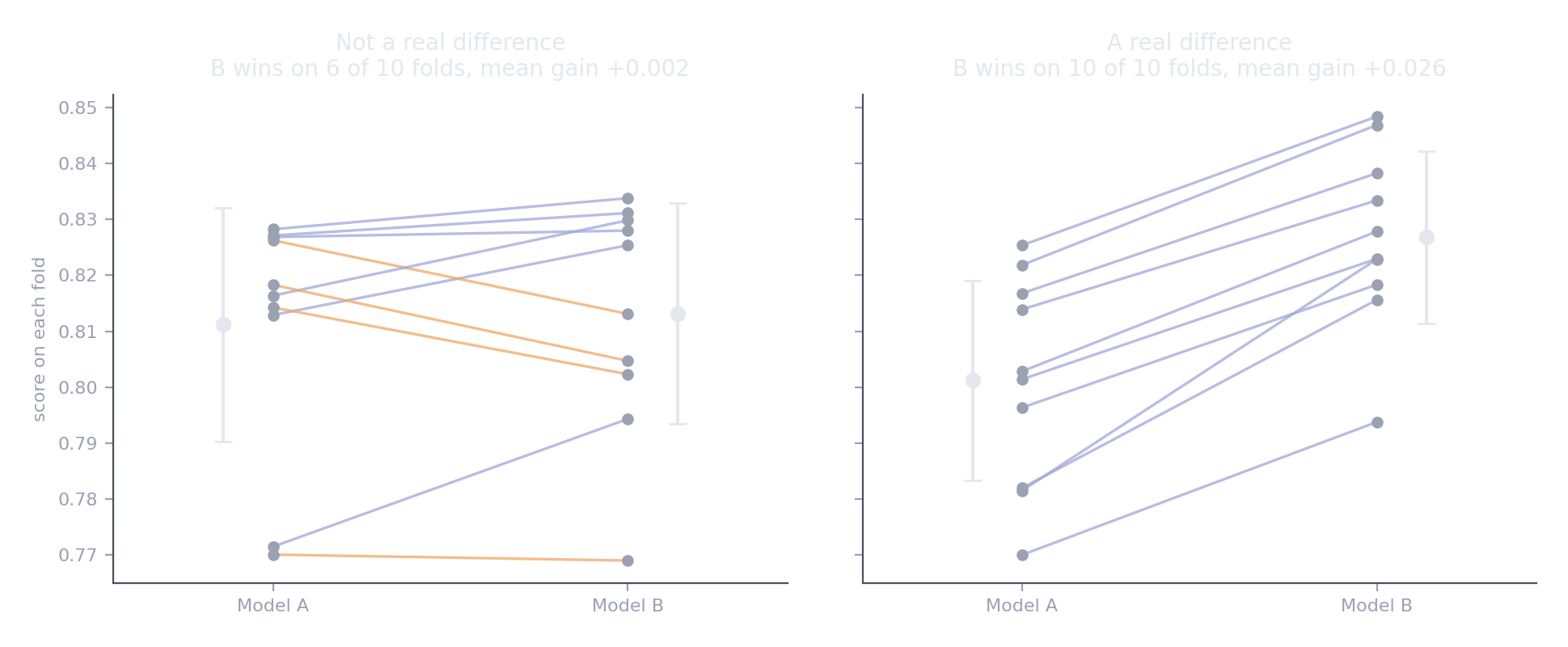
Each line is one fold, joining model A's score to model B's. Black markers show mean and standard deviation. On the right the error bars overlap heavily, yet B wins on every single fold. The averages alone would not convince you. The pairing does.
from sklearn.model_selection import RepeatedStratifiedKFold, cross_val_score

cv = RepeatedStratifiedKFold(n_splits=5, n_repeats=5, random_state=42)

a = cross_val_score(model_a, X, y, cv=cv, scoring="roc_auc")
b = cross_val_score(model_b, X, y, cv=cv, scoring="roc_auc")
diff = b - a      # same cv object, same seed, so the folds match

print(f"A: {a.mean():.3f} ± {a.std():.3f}")
print(f"B: {b.mean():.3f} ± {b.std():.3f}")
print(f"B wins on {(diff > 0).sum()} of {len(diff)} folds, mean gain {diff.mean():+.3f}")
Repeating the cross-validation five times gives 25 paired comparisons instead of 5, which makes the win count far more informative.
For a single held-out test set, bootstrap the difference instead: resample the test rows with replacement many times and see how the gap moves.
rng = np.random.default_rng(42)
n = len(y_test)
gaps = []
for _ in range(2000):
    idx = rng.integers(0, n, n)
    gaps.append(score(y_test[idx], pred_b[idx]) - score(y_test[idx], pred_a[idx]))

low, high = np.percentile(gaps, [2.5, 97.5])
If that interval includes zero, you cannot claim B is better.
Rules for writing it up
- If the mean gain is smaller than the fold-to-fold standard deviation, and the wins are split, do not claim a difference.
- Write "B beat A on 23 of 25 folds by an average of 0.012 AUC", not "B is better". The first is a finding. The second is an opinion.
- Folds share training data, so they are not truly independent, and these spreads understate the real uncertainty. Treat every result as slightly optimistic, which is one more reason to claim less.
9. Calibration
A classifier that outputs 0.8 is saying: of all the cases I give 0.8, about 80% should turn out positive. A calibrated model keeps that promise.
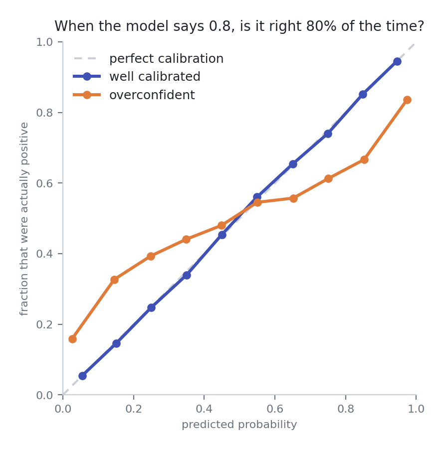
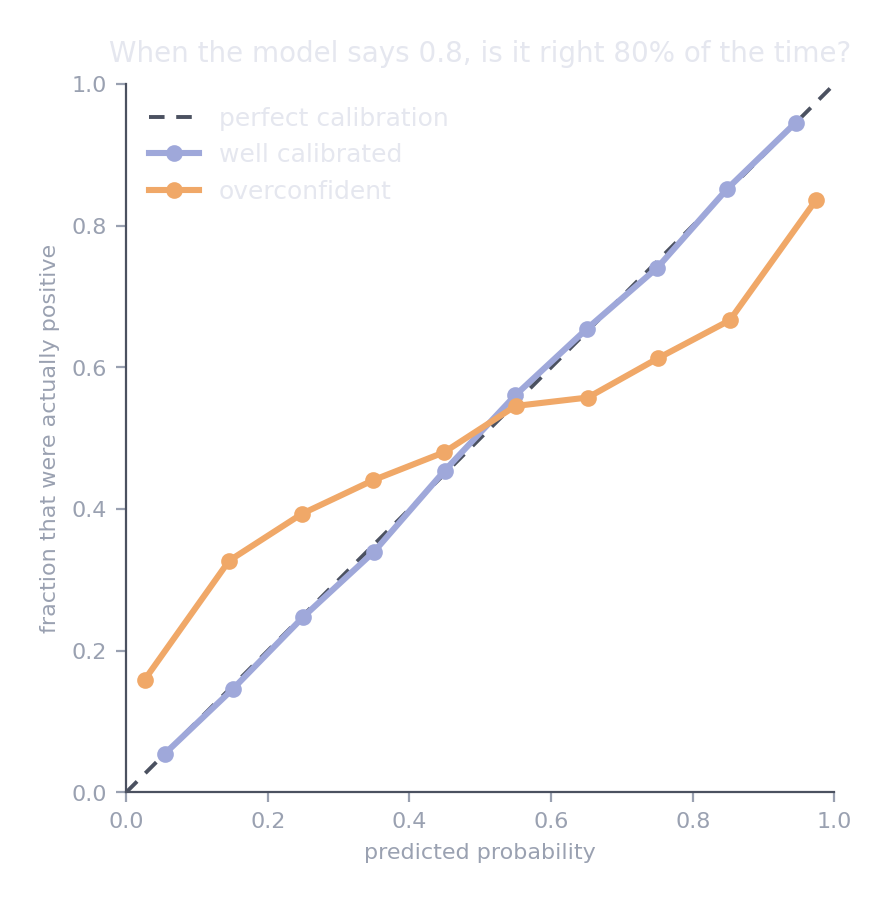
Group predictions into bins, then check how often each bin was actually positive. The overconfident model pushes its probabilities towards 0 and 1 further than reality justifies.
Logistic regression is often reasonably calibrated out of the box. Tree ensembles, boosting, and support vector machines frequently are not. It matters whenever the probability itself drives a decision, such as choosing a threshold or estimating an expected cost. If you only care about ranking, it matters much less.
from sklearn.calibration import CalibrationDisplay, CalibratedClassifierCV

CalibrationDisplay.from_estimator(model, X_test, y_test, n_bins=10)

calibrated = CalibratedClassifierCV(model, method="isotonic", cv=5).fit(X_train, y_train)
Where this lands
Week 9, where calibration is one of the three things model selection asks you to check.
What this page skips
Quick reference
| Concept | In one line |
|---|---|
| Standard error | \(\sigma / \sqrt{n}\). Noise in an average shrinks with the square root of the sample size. |
| i.i.d. | What a random split assumes. Break it and the score flatters you. |
| Precision | \(P(\text{real} \mid \text{flagged})\) |
| Recall | \(P(\text{flagged} \mid \text{real})\) |
| Base rate | A rare class makes accuracy meaningless |
| Paired comparison | Same folds for both models, then count the wins |
| Bootstrap | Resample rows with replacement to see how much a score moves |
| Calibration | Does a predicted 0.8 come true 80% of the time? |
| Task | Code |
|---|---|
| Log-transform a skewed target | np.log1p(y), then np.expm1(pred) |
| Repeated cross-validation | RepeatedStratifiedKFold(n_splits=5, n_repeats=5, random_state=42) |
| Reliability diagram | CalibrationDisplay.from_estimator(model, X, y) |
| Recalibrate | CalibratedClassifierCV(model, method="isotonic") |
Resources
- Seeing Theory, Brown University. Interactive visual introduction to probability. The fastest way to rebuild intuition.
- An Introduction to Statistical Learning, chapter 5 on resampling methods. Free PDF, and the clearest account of cross-validation and the bootstrap.
- Sebastian Raschka, Model Evaluation, Model Selection, and Algorithm Selection in Machine Learning. The thorough version of section 8, for when you want to go further than this page does.
- Think Stats, Allen Downey. Free, practical, written in Python.
Next in this section: Choosing a metric, which picks up where sections 5 and 6 leave off.