Linear Algebra for ML
At a glance
You need this in: Week 05 (linear models), Week 07 (regularization), Week 11 (PCA) Estimated time: 35 minutes Assumed: you have seen matrices before, even if it was a while ago
This page is not a linear algebra course. It covers the handful of ideas that appear in this course's lectures and code, in the order they appear, each one tied to the place it lands.
If the notation in a Week 5 slide is the problem, this page is the fix. If you want to properly learn the subject, the resources at the bottom are better than anything here.
1. A vector is a row of your dataframe
Forget arrows for a moment. In this course a vector is one observation, written as a list of numbers.
Every apartment in your dataset is a point in four-dimensional space. You cannot picture that, and you do not need to. Everything that works in two dimensions works in four hundred, which is the whole reason this notation is worth learning.
2. The dot product is a prediction
Multiply matching entries, add them up.
That line is a linear regression. When Week 5 writes \(\hat{y} = \mathbf{w}^\top \mathbf{x} + b\), it means exactly what that code does: weight each feature by how much it matters, add them, add an offset.
Where this lands
Week 5. Once you see that a linear model is a dot product, coefficients stop being mysterious. A weight of 1200 on area means one extra square metre adds 1200 to the prediction, holding everything else fixed.
3. A matrix is your whole dataset
Stack every observation as a row and you have the design matrix, universally called \(X\).
This is why scikit-learn insists on a 2D array. Rows are observations, columns are features, always, without exception. When something fails with a shape error, check that you have not transposed this by accident.
4. Matrix times vector predicts everything at once
Both give the same answer. The first runs in compiled code on the whole array at once, and on a real dataset it is a hundred times faster. Vectorization is not a performance trick bolted on afterwards, it is what the notation was designed for.
5. Shapes, and how to debug them
One rule governs every matrix multiplication:
The inner dimensions must match and they vanish. The outer ones survive.
The trap that will catch you in a lab
(100,) and (100, 1) are not the same thing. The first is a one-dimensional array, the second is a matrix with one column. NumPy will sometimes broadcast between them and silently give you a (100, 100) result instead of the (100,) you expected.
a = np.zeros(100)         # (100,)
b = np.zeros((100, 1))    # (100, 1)
(a - b).shape             # (100, 100)  almost never what you wanted
When an ML operation misbehaves, print the shapes before anything else:
Use .reshape(-1) to flatten and .reshape(-1, 1) to make a column.
6. Transpose, and why \(X^\top X\) is everywhere
Transposing flips rows and columns.
The product \(X^\top X\) has shape \((4, 4)\): one row and column per feature. It is, up to scaling, the covariance structure of your features, and it turns up in the least squares solution, in ridge regression, and in PCA. When you see it, read it as "how the features relate to each other."
7. Norms measure size, and they become regularization
A norm is the length of a vector. Two of them matter here.
np.linalg.norm(w)          # L2, ordinary Euclidean length
np.linalg.norm(w, ord=1)   # L1, sum of absolute values
Where this lands
Week 7, and this is the shortest path to understanding regularization.
Ridge adds \(\lambda\|\mathbf{w}\|_2^2\) to the loss, so large weights are expensive and everything gets shrunk toward zero together.
Lasso adds \(\lambda\|\mathbf{w}\|_1\). Because of the shape of the L1 ball, the cheapest way to reduce that penalty is often to set a weight to exactly zero. That is why lasso selects features and ridge does not.
Distance between two observations uses the same L2 norm, which is how k-nearest-neighbours and k-means decide what is close.
8. Least squares is a projection
Here is the geometric picture that makes linear regression click.
Your target \(\mathbf{y}\) is a vector. The columns of \(X\) span a subspace, the set of every prediction your model is capable of producing. Usually \(\mathbf{y}\) does not lie in that subspace, so you cannot predict it exactly.
Least squares finds the closest point that you can reach, which is the perpendicular projection of \(\mathbf{y}\) onto that subspace.
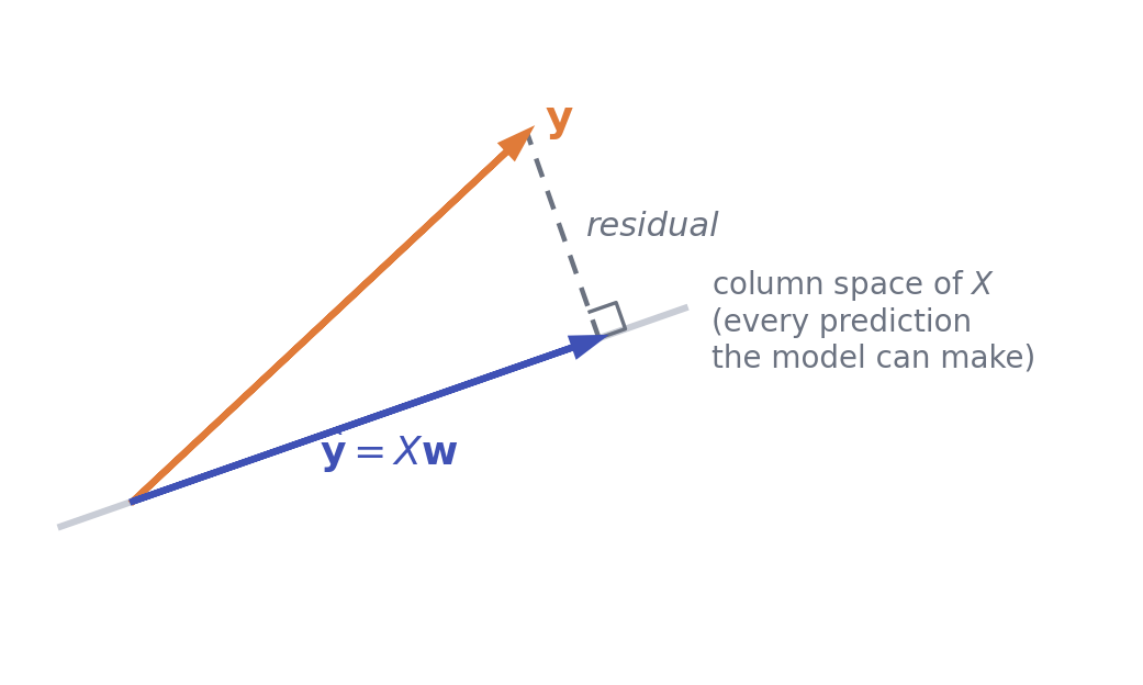
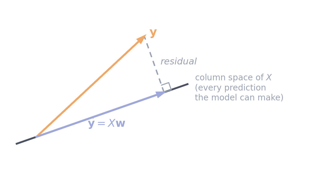
The residual is perpendicular to everything the model can express. That is what "best fit" means geometrically.
The residual being perpendicular is not a coincidence, it is the condition that defines the solution. Write it out and you get the normal equations:
Never invert a matrix if you can solve instead
np.linalg.solve is faster and numerically far more stable than forming an explicit inverse. The formula above is written with an inverse because that is how it is derived, not because it is how you compute it.
9. Eigenvectors, briefly
Most vectors change direction when you multiply them by a matrix. A few only get stretched.
Those special directions are eigenvectors, and \(\lambda\) is how much each one is stretched. That is the whole idea, and this course needs it for exactly one purpose: the eigenvectors of the covariance matrix are the directions your data varies in most.
10. SVD, and why PCA is just SVD
Every matrix factors into three pieces.
The columns of \(V\) are directions in feature space. The diagonal entries of \(\Sigma\) say how much the data spreads along each one, in decreasing order. So the first column of \(V\) is the single direction that captures the most variance in your dataset, the second is the best remaining direction perpendicular to it, and so on.
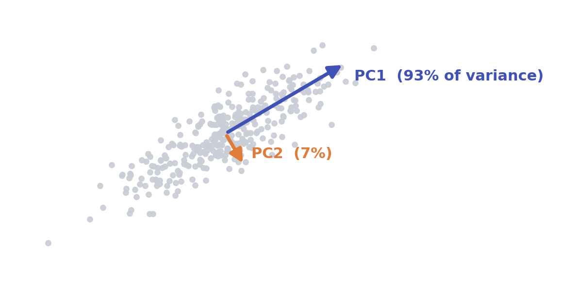
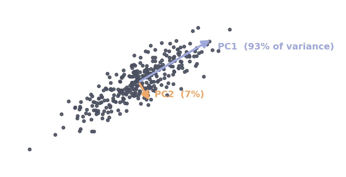
Correlated data with the two directions the SVD finds. PC1 is the single direction holding most of the variance, PC2 is the best remaining direction at right angles to it.
X_centred = X - X.mean(axis=0)          # centring is not optional
U, S, Vt = np.linalg.svd(X_centred, full_matrices=False)

variance_explained = S**2 / np.sum(S**2)
X_2d = X_centred @ Vt[:2].T             # project onto the top two directions
Where this lands
Week 11. PCA is this and nothing more. When sklearn.decomposition.PCA runs, it centres your data and calls an SVD. Knowing that is why you will understand why centring matters, why scaling changes the answer, and why the components are orthogonal.
What this page skips
Left out on purpose, so you know these are not gaps you need to fill for this course.
Quick reference
| You want | NumPy |
|---|---|
| Dot product | a @ b or np.dot(a, b) |
| Matrix product | A @ B |
| Transpose | A.T |
| Shape | A.shape |
| Flatten to 1D | a.reshape(-1) |
| Make a column | a.reshape(-1, 1) |
| L2 norm | np.linalg.norm(w) |
| L1 norm | np.linalg.norm(w, ord=1) |
| Solve a linear system | np.linalg.solve(A, b) |
| SVD | np.linalg.svd(X, full_matrices=False) |
| Eigen-decomposition | np.linalg.eig(A) |
| Column means | X.mean(axis=0) |
| Shape rule | |
|---|---|
(n, k) @ (k, m) |
gives (n, m) |
(n, k) @ (k,) |
gives (n,) |
(n,) vs (n, 1) |
different, and the cause of most shape bugs |
Resources
- 3Blue1Brown, Essence of Linear Algebra. Fifteen short videos, and the best intuition anyone has built for this material. If one section above did not land, the corresponding video almost certainly will.
- Mathematics for Machine Learning, chapters 2 to 4. Free PDF, and the proper treatment of everything here.
- NumPy linear algebra docs for the full function list.
Next in this section: Calculus for ML, which covers how a model actually learns the weights this page assumed it already had.