Week 03 · Feature engineering

At a glance

Block: 1 · Data & the Pipeline Running example: Olist orders. Will this order arrive late? New to it? Start with the Block 1 overview. Lab: week-03/lab.ipynb in the labs repository Before class: read sections 1, 3 and 5, about fifteen minutes

Why this matters

Good features beat clever algorithms. A leaky feature beats nothing at all, until the day it meets real data.

Last week ended badly. Judged on the future, Week 1's baselines were barely better than guessing. The model was never the problem: the features were. This week you build better ones, from what exists at the moment of prediction, and you build them inside a structure that makes leaking hard to do by accident.

Two things make this week different from simply "adding columns". Some features are computed from a single row and are safe anywhere. Others are learned from many rows, and those are where the quietest leaks in machine learning live. Telling the two apart is most of the skill.

This week at a glance

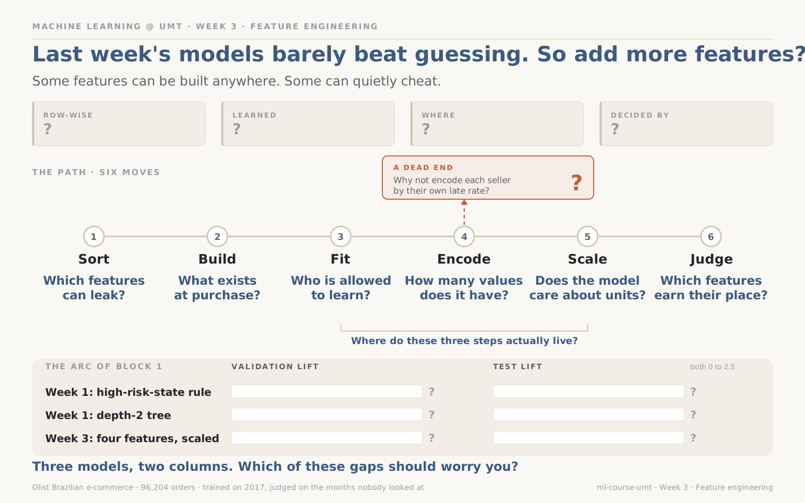
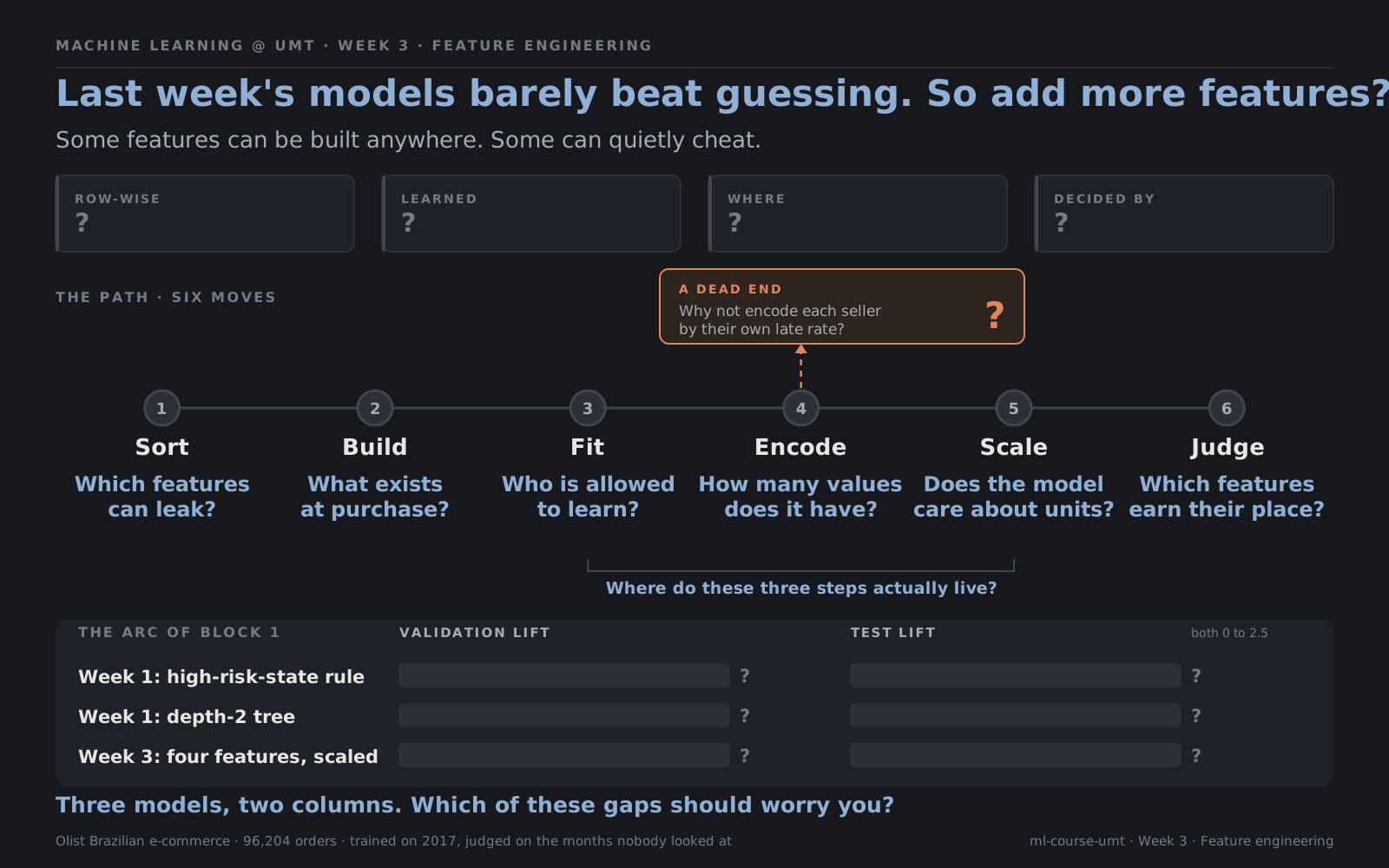
Six moves, and the question each one asks. Three of them only make sense inside the same pipeline, which is what the bracket marks.

Sections 1 to 4 are about building features safely. Sections 5 to 7 put them into one pipeline with the model. Section 8 decides which ones stay.

Learning outcomes

By the end of this week you can:

• Tell a row-wise feature from a learned one, and say which can leak
• Build features from what exists at the moment of prediction
• Spot a statistic computed over the whole dataset, and fix it
• Write a scikit-learn transformer with fit and transform
• Put preprocessing and model into one pipeline with a ColumnTransformer
• Choose an encoding for a category based on how many values it has
• Decide when scaling matters, and read a scaled model's coefficients
• Judge each feature on validation, and look at test exactly once

Before class

Bring an answer

A music app predicts whether you will skip a song. It could use "how often you skip songs" or "how often everyone skips this song". Which of those two needs more care when you build it, and why?

---

1. Know the two kinds of feature

Every feature you will ever build is one of two kinds, and the difference decides whether it can leak.

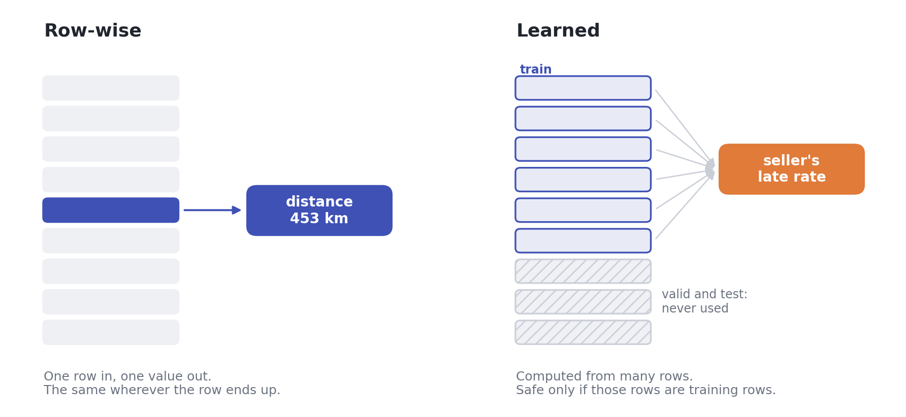
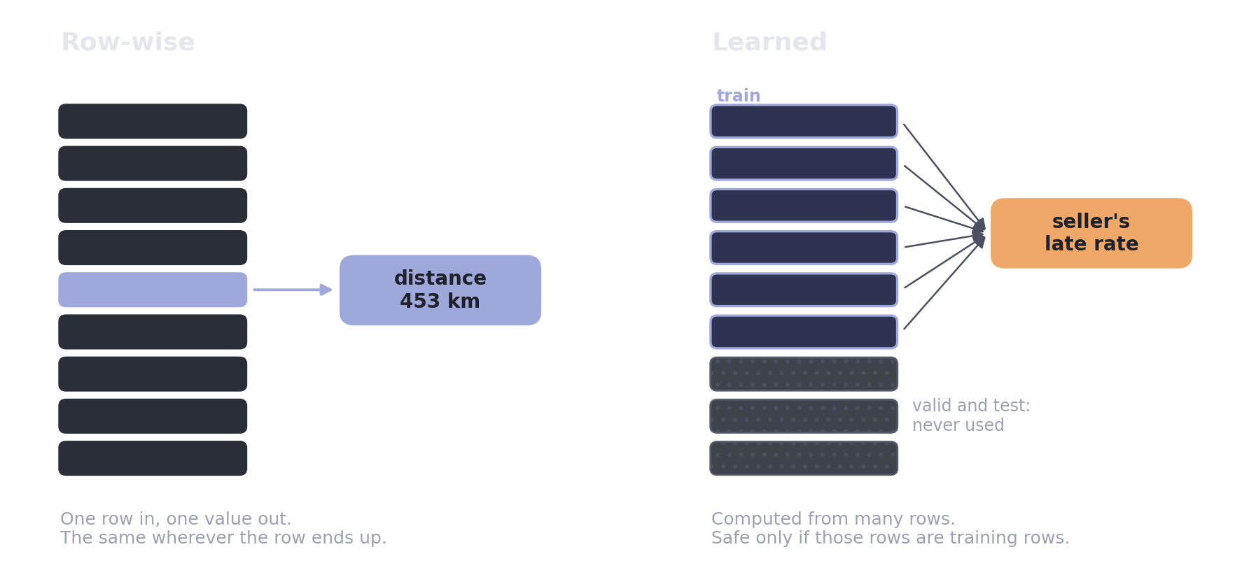
Row-wise features are computed from one row on its own: a distance, a ratio, a flag, the day of the week. The value for a row is the same whether that row lands in training or in test. They cannot leak through the split, so you can build them before or after it.

Learned features are computed from many rows: an average, a typical value, a rate per category. The value for a row depends on which other rows were used. If those include test rows, the feature carries information from the test set into training. Learned features must be computed from training rows only, after the split.

Key insight

Ask of every feature: could its value change if I split the data differently? If yes, it is learned, and it belongs after the split, fitted on training rows only.

In our example

Feature	Kind
Distance from seller to customer	Row-wise
Same state or not	Row-wise
Days promised	Row-wise
Freight as a share of price	Row-wise
Typical delivery time on this route	Learned
The seller's late rate	Learned
The category's late rate	Learned

Elsewhere: in credit scoring, "this applicant's debt divided by their income" is row-wise. "How this applicant's income compares with the average in their region" is learned.

In your project

List every feature you plan to build, and label each one row-wise or learned. The learned ones get extra care for the rest of this week.

2. Build features from what exists at prediction time

Good features usually come from understanding the problem, not from clever transformations. A few families cover most of what you will need:

Family	Examples
Distances and differences	Kilometres between two points, days between two dates
Ratios	Cost per unit, debt per income, freight per price
Flags	Same region or not, first order or not, weekend or not
Parts of dates	Weekday, month, hour, days until a holiday
Counts and totals	Items in a basket, visits in the last month

Every one must pass Week 1's test: does this value exist at the moment of prediction?

Before any model, test each new feature on its own. Use it alone as a score and measure its lift on validation. A feature that says nothing alone may still help in combination, but a quick look tells you where the signal is.

In our example

Four row-wise features, each from one row: distance_km (using the haversine formula, the straight-line distance on a sphere), same_state, window_days, and freight_ratio. The typical order travels about 450 km, a third stay within one state, and freight costs about a fifth of the price.

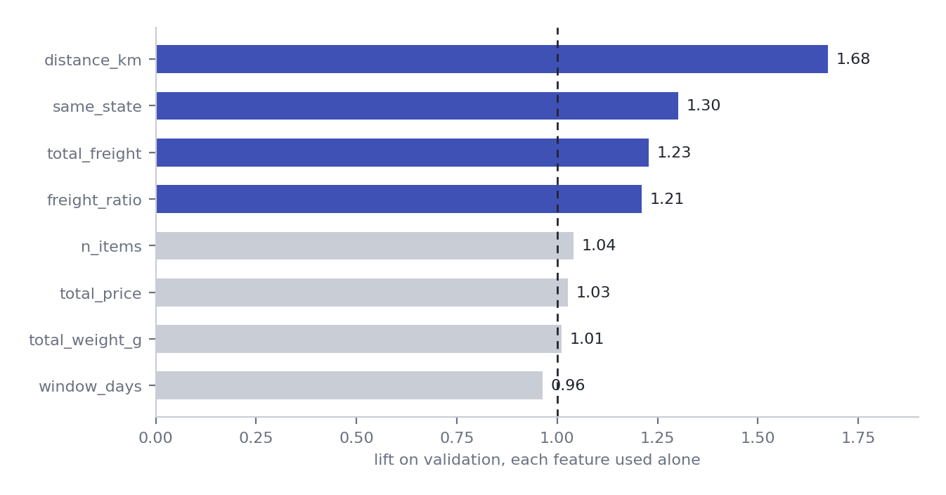
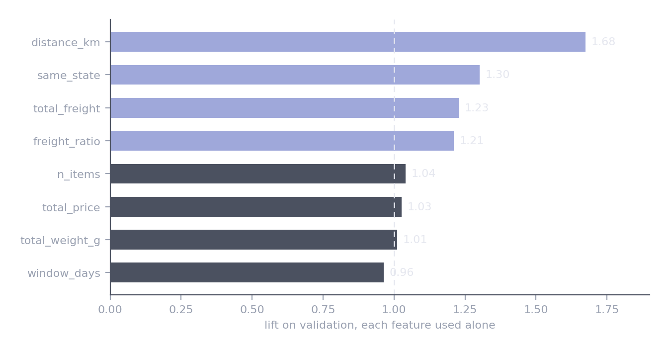
Distance says the most on its own. Weight, price, basket size, and the length of the promise say almost nothing alone. Section 7 shows why "alone" is not the whole story.

Elsewhere: for predicting whether a flight is delayed, the distance of the route, the hour of departure, and whether it is the last flight of the day are all row-wise and all available at booking.

In your project

Build at least three row-wise features from your domain, and test each one alone on validation. Keep the table: it is a useful record of where the signal is.

3. Fit learned features on training data only

The quietest leak in machine learning is a statistic computed over the whole dataset. It looks like good practice: more data, more reliable averages. But if the average for a group includes test rows, then each test row's own answer is already inside the feature it is judged with.

The rule is short: anything learned from many rows is learned from the training rows, and only applied to the others.

That rule reaches further than it first looks, because it is not only about features you set out to build. Filling a missing weight with the median learns a median. A scaler stores a mean and a standard deviation. An encoder remembers which categories it saw. All three are learned from rows, so all three belong after the split, fitted on training rows alone, which is exactly why they end up inside the pipeline in section 5.

Missing values are the most common of the three. Two Olist products have no weight, and SimpleImputer(strategy="median") fills them from the median of the training rows. That one number is then stored and applied unchanged to validation and to test: the test rows never get a median of their own.

In our example

Some sellers are late far more often than others, so a seller's late rate sounds like an excellent feature. The only question is which orders it is computed from.

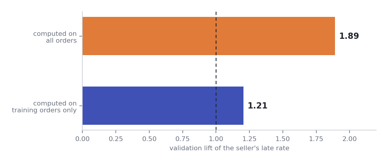
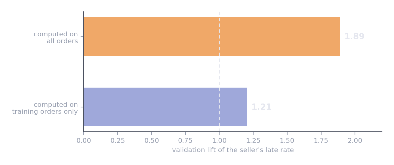
The same feature, scored on the same validation orders. The only difference is where the rate was computed.

Computed from all orders, validation orders' own labels sit inside their sellers' averages, and the feature scores 1.89. Computed honestly, from training orders only, it scores 1.21.

It looks like a good feature

No error, no warning, and a score that improves. This is the leak Week 1 promised: much quieter than using the delivery date, and much easier to make.

Elsewhere: a hospital builds "readmission rate of this doctor" from all its records, test patients included. The feature looks powerful in evaluation and disappoints on new patients.

In your project

For every learned feature, write down which rows it is computed from. If the answer is anything other than "training rows only", fix it before going further.

4. Transformers: fit learns, transform applies

The fix for learned features is not a trick. It is a pattern, and every preprocessing step in scikit-learn follows it. A transformer has two methods:

• fit learns something from training data and stores it, in attributes whose names end with an underscore
• transform applies what was learned, to any data

flowchart LR
    T["<b>Training rows</b>"] -->|fit| S["<b>What was learned</b><br/>medians, rates, categories<br/>stored in attributes ending in _"]
    S --> X{{"transform"}}
    T2["Training rows"] --> X
    V["Validation rows"] --> X
    N["New orders"] --> X
    X --> F["<b>Features</b>"]

Learning happens once, on training data. Applying happens everywhere. fit_transform is a shortcut for both on the same data, which is exactly why it is only ever called on training data.

There is one more rule, and it matters most: fit may look at the past, including outcomes, because it only sees training data. transform may only use what exists at the moment of prediction, because it will run on new cases where the outcome has not happened yet.

In our example

Olist pads its promises, so a useful question is how much slack a promise leaves compared with the typical delivery time on that route. The typical time must be learned, so it goes in fit:

class RouteSlack(BaseEstimator, TransformerMixin):
    def fit(self, X, y=None):
        days_taken = (X["order_delivered_customer_date"].dt.normalize()
                      - X["order_purchase_timestamp"].dt.normalize()).dt.days
        route = X["seller_state"] + " > " + X["customer_state"]
        self.typical_days_ = days_taken.groupby(route).median()     # learned from the past
        self.overall_days_ = days_taken.median()
        return self

    def transform(self, X):
        route = X["seller_state"] + " > " + X["customer_state"]
        typical = route.map(self.typical_days_).fillna(self.overall_days_)
        promised = (X["order_estimated_delivery_date"]
                    - X["order_purchase_timestamp"].dt.normalize()).dt.days
        return pd.DataFrame({"slack_days": promised - typical}, index=X.index)   # no delivery date here

Fitted on training orders, it learns 369 routes. A typical São Paulo to Rio parcel takes 13 days, and the median promise leaves 11 days of slack beyond the typical trip.

Elsewhere: a transformer that learns the typical price per square metre in each neighbourhood, from past sales, and then computes how a new listing's asking price compares with it.

In your project

Write at least one learned feature as a transformer class. Check two things: fit stores everything it learns in attributes ending in _, and transform never reads a column that would not exist at prediction time.

5. Pipelines make leakage structurally impossible

Doing each step by hand is how leaks creep in. One fit on the wrong data is enough, and it is easy to make in a long notebook. A pipeline removes the chance. It holds every preprocessing step and the model in one object:

• pipeline.fit(train) fits every step, in order, on training data only
• pipeline.predict(anything) applies every step using only what was learned during fit

Different columns need different treatment, so a ColumnTransformer routes each group of columns to its own steps and joins the results.

In our example

flowchart LR
    D["<b>Order table</b>"] --> CT
    subgraph CT["ColumnTransformer"]
        direction TB
        NUM["<b>8 numbers</b><br/>fill gaps with the median, then scale"]
        ST["<b>2 states</b><br/>one-hot encode"]
    end
    CT --> M["<b>Logistic regression</b>"]
    M --> P["<b>Probability of arriving late</b>"]

numeric = Pipeline([("impute", SimpleImputer(strategy="median")), ("scale", StandardScaler())])

prep = ColumnTransformer([
    ("numeric", numeric, ROW_WISE),
    ("states", OneHotEncoder(handle_unknown="ignore"), ["customer_state", "seller_state"]),
])

model = Pipeline([("prep", prep), ("model", LogisticRegression(max_iter=2000, class_weight="balanced"))])
model.fit(train, train["is_late"])

Validation lift 2.34, against 1.57 and 1.65 for Week 1's baselines on the same data. The imputer's medians and the scaler's means were learned from training orders, inside the pipeline, without a single line of code that could have used the wrong rows.

Elsewhere: a pipeline is also what you deploy. Save the fitted pipeline, and a new record goes in raw and comes out as a prediction, transformed with exactly the statistics the model was trained with.

In your project

Put every preprocessing step and your model into a single pipeline. A good test: your notebook should contain no call to fit or fit_transform outside the pipeline.

6. Encode categories by how many values they have

Models need numbers, so every category has to be encoded. The right encoding depends mostly on how many different values the column has:

Values	Encoding	Watch out for
A handful, unordered	One-hot: one column per value	Nothing much. The default.
A handful, with a real order	Ordinal: small, medium, large becomes 0, 1, 2	Only when the order is genuine
Many	Target encoding: each value becomes the average target for that value	Must be cross-fitted, or the model trusts it far too much
An ID per entity	Often better left out	Thousands of values, most seen only a few times
Free text	Word counts or TF-IDF, which turn words into weighted counts	Only text that exists at prediction time

Ordinal encoding is the one people reach for first, because it is the least typing: give each category a number and carry on. It is right when the categories really do have an order, poor, fair, good or small, medium, large, because then "a bigger number means more" is true and the model can use it. It is wrong the rest of the time, and quietly so. Number the Brazilian states 0 to 26 and a linear model will happily conclude that state 20 is worth twice state 10. One-hot costs you columns and saves you that.

Two names worth separating: in scikit-learn, OrdinalEncoder is for feature columns and LabelEncoder is for the target. They do nearly the same thing, which is why LabelEncoder ends up on a feature column often enough to be worth warning about.

Target encoding is a learned feature, so it must come from training rows. But there is a second trap. If each training row is encoded with an average that includes its own label, the model sees a feature that is partly the answer, and learns to trust it far too much. The fix is cross-fitting:

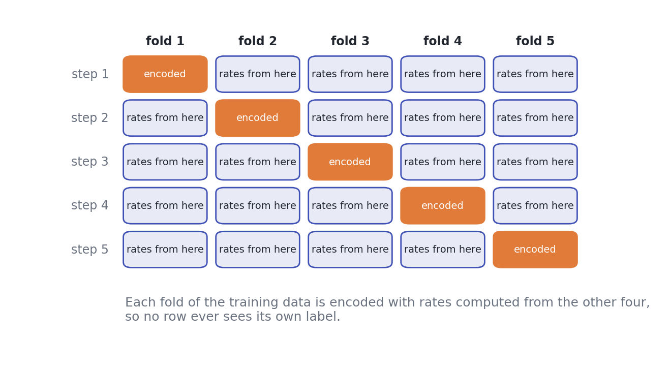
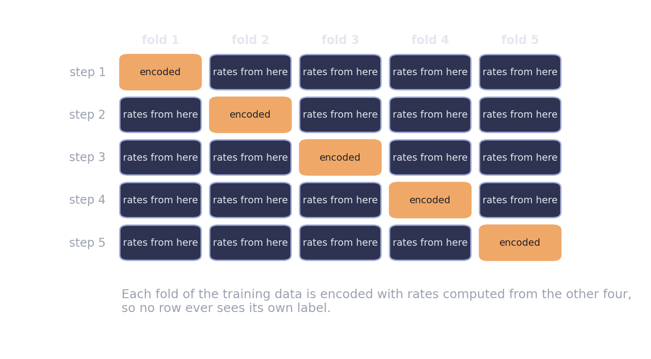
scikit-learn's TargetEncoder does this for you inside fit_transform, which is one more reason to keep it in a pipeline.

In our example

States have 27 values, so they are one-hot encoded. Sellers have almost 3,000. Encode them naively, with rates computed on the same training rows, and compare with cross-fitting:

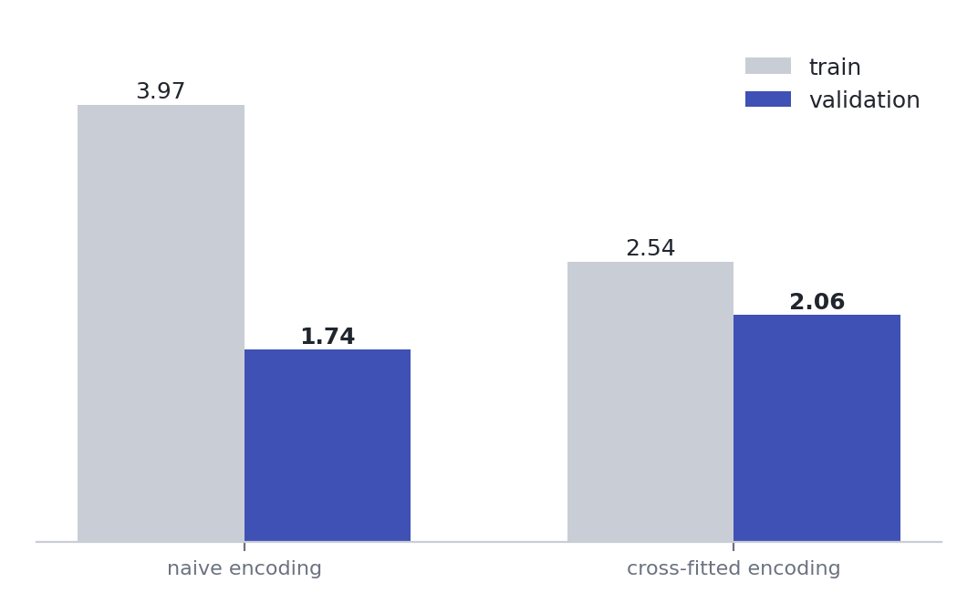
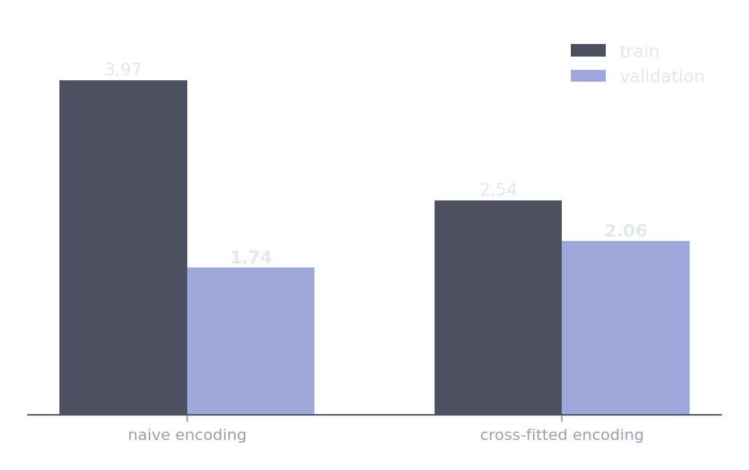
Naive encoding looks brilliant on training data, 3.97, and falls to 1.74 on validation. Cross-fitting gives a lower training score and a higher validation score: the gap shrinks because the model is no longer fooled by its own labels.

Olist has no text that exists at the moment of purchase: the only free text is in reviews, which are written after delivery. So there is no TF-IDF in this week's model. The scikit-learn cheatsheet shows how to use it when your data has text.

The category nobody has seen before

An encoder is fitted on training rows, so it knows only the categories that were in them. A city, a seller or a product type that turns up for the first time in production is not a rare edge case, it is routine, and the time to decide what happens is before it happens. OneHotEncoder(handle_unknown="ignore") turns an unknown value into all zeros instead of raising an error, and TargetEncoder falls back to the overall average. The scikit-learn cheatsheet has the settings.

Elsewhere: a postcode with 20,000 values, a product ID, a doctor's name. All tempting, all high-cardinality, and all worth asking whether the model can really learn from them.

In your project

Count the distinct values in each categorical column. Choose one-hot, cross-fitted target encoding, or leaving it out, and write one line explaining each choice.

7. Scale when the model cares

Some models are sensitive to the scale of their inputs, and some are not:

Model	Needs scaling?	Why
Logistic and linear regression	Yes	Trained by gradient steps, which struggle when features differ wildly in scale
Anything based on distances	Yes	A feature in thousands would drown out one in units
Decision trees and their ensembles	No	They split on thresholds, and a threshold does not care about units

Standardising, the usual choice, means subtracting the mean and dividing by the standard deviation, so each feature ends up centred near zero with a spread of about one. Both of those numbers are learned from the training rows, which makes the scaler one more step that belongs inside the pipeline. Two alternatives are worth knowing: MinMaxScaler squeezes everything into the range 0 to 1, useful when a bounded range matters, and RobustScaler uses the median and the interquartile range instead, which is the one to reach for when a handful of extreme values would drag the mean around.

The calculus page shows what goes wrong for gradient descent when features are badly scaled. There is a second reward: once every feature is on the same scale, the coefficients of a linear model become comparable, and the model becomes readable.

In our example

Without the scaler, logistic regression runs out of steps before it finds its best weights: it stops with a convergence warning, and validation lift drops from 2.34 to 2.28. Scaled, the coefficients tell a clear story:

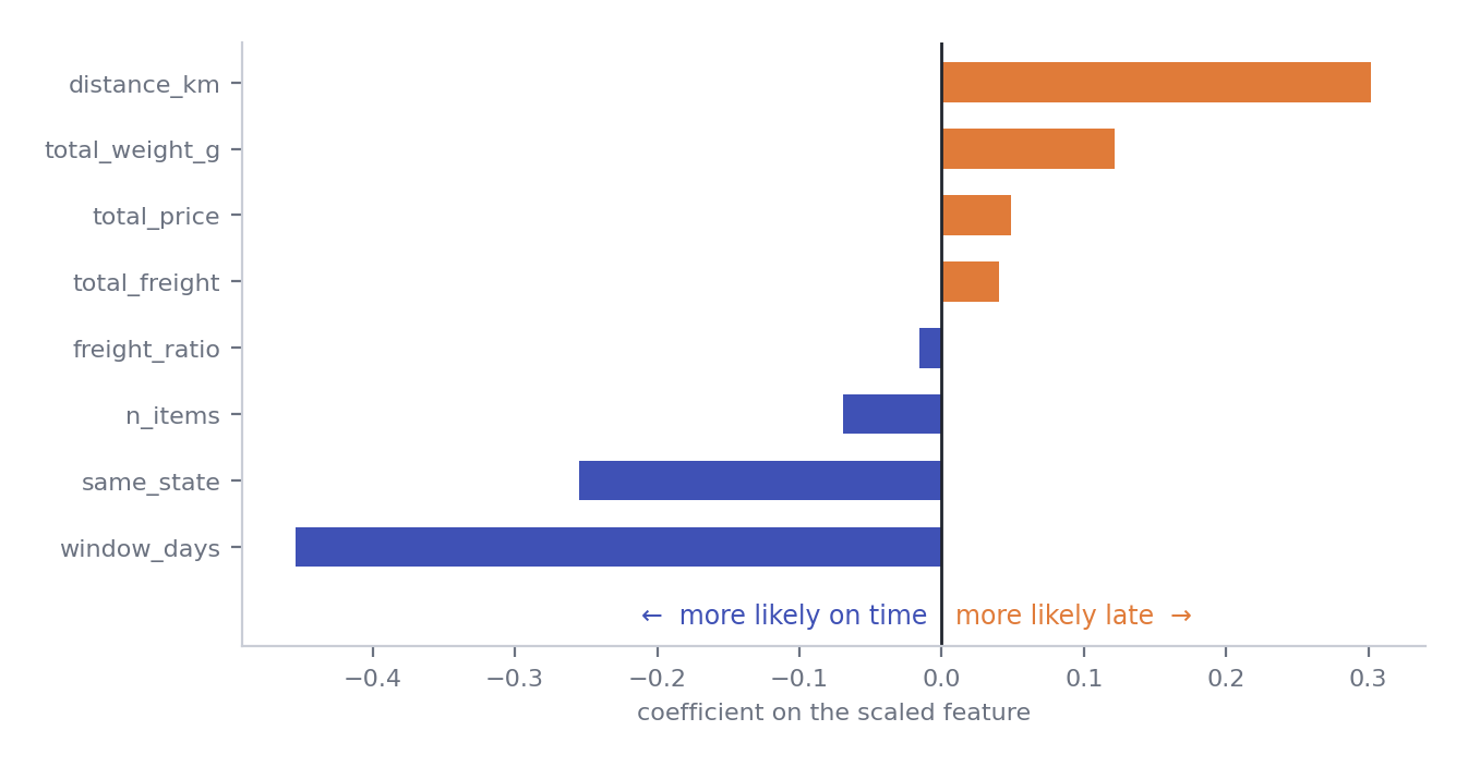
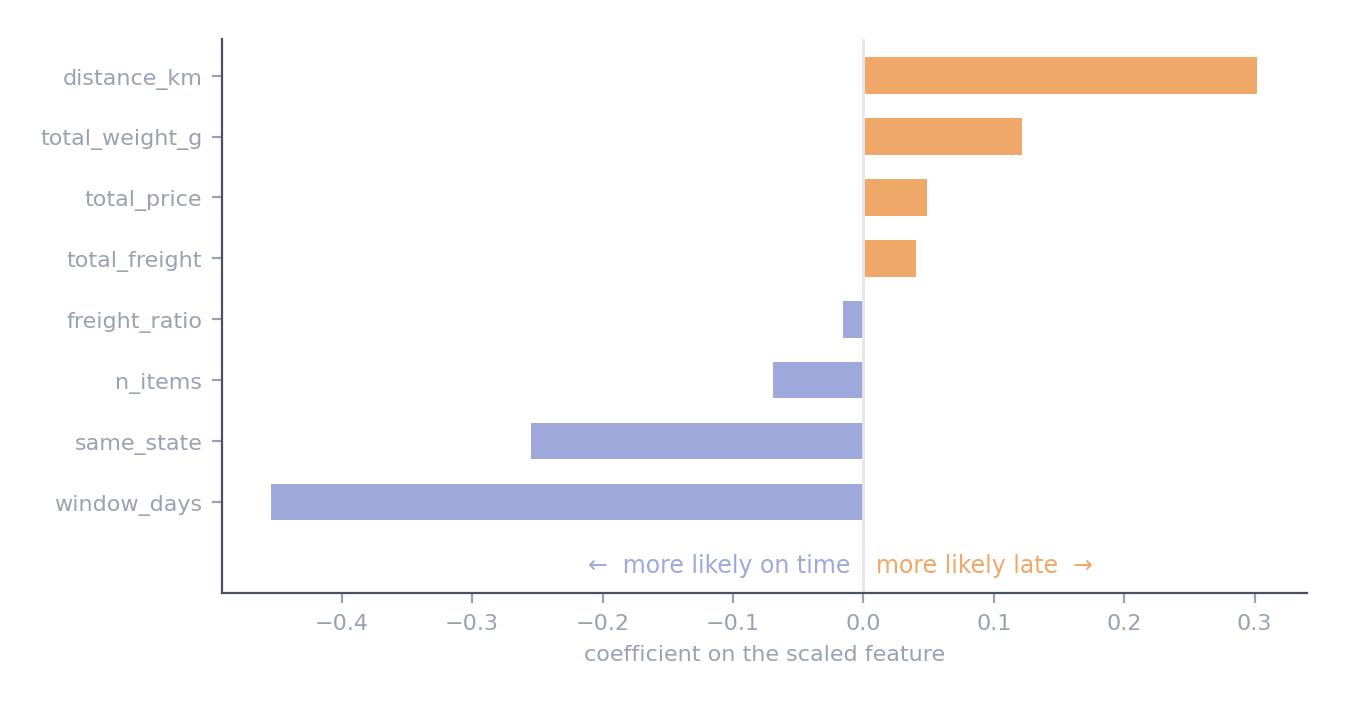
A longer promise pushes hardest towards on time. Distance pushes towards late, and staying within one state towards on time.

Look at window_days. On its own, in section 2, it was the weakest feature. In the model, it has the strongest coefficient. A long promise only means something once the model also knows how far the parcel travels. Useless alone does not mean useless in a model.

In your project

If you use a linear model, scale its numeric inputs inside the pipeline, then plot the coefficients. If any of them contradicts what you know about the domain, find out why before trusting the score.

8. A feature must earn its place

More features are not automatically better. Each one adds a way to overfit, a column to maintain, and a possible leak. So every candidate has to earn its place, with a simple protocol:

1. Start from a solid base model
2. Add one candidate, or one group, at a time
3. Judge each on validation, never on test
4. Keep only what clearly helps
5. When every decision is made, score the final model on test, once

In our example

Three learned candidates on top of the row-wise model, plus the same features in a tree:

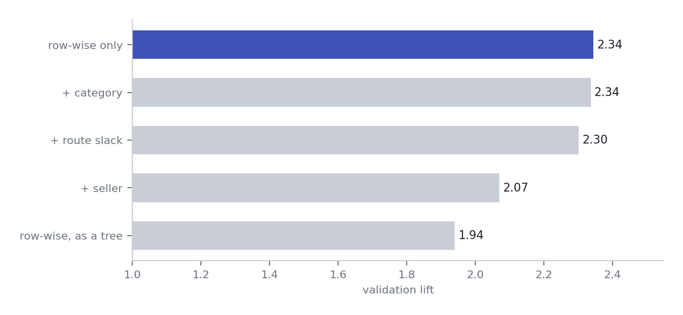
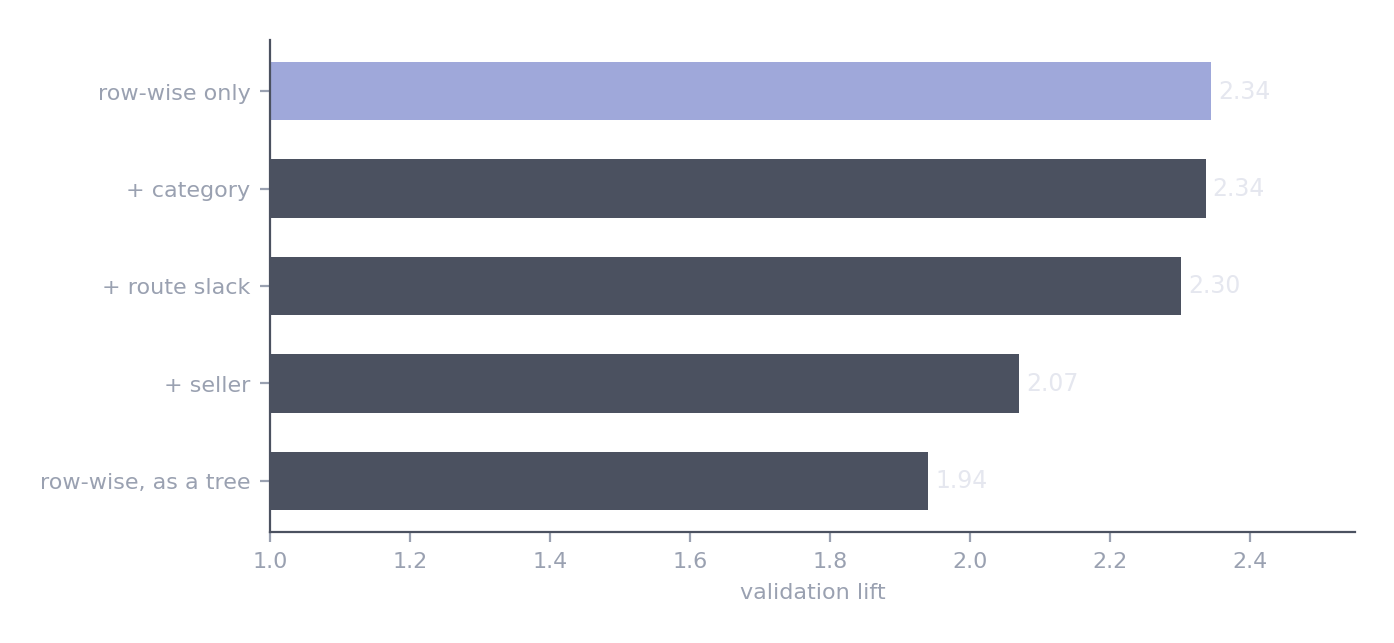
None of the learned features clearly beats the plain row-wise model. The category ties, the route slack and the seller make validation worse, and the tree loses on the same features.

The simplest model wins, so it is the one we keep. Then, and only then, one look at test: a lift of 1.87, against 1.10 and 1.18 for Week 1's baselines on the same future months. Lower than the 2.34 on validation, as Week 2 led us to expect, since the test months are calmer. But the gain is real, and it held on data nobody looked at while choosing.

Key insight

A clever feature that loses on validation is a lesson, not a failure. You know the simpler model is better because you tested it on data it never saw, not because it felt right.

Elsewhere: a churn team adds forty engineered features and gains nothing on validation. The honest report says so, and ships the model with eight. It is easier to explain, cheaper to run, and just as good.

In your project

Run the protocol: a base model, then each candidate on its own, judged on validation. Report every result, including the features that lost, then score the chosen model on test once.

---

Lab

Lab · week-03/lab.ipynb

In the labs repository. You write most of the code yourself, and it runs longer than one session on purpose: parts 5 to 7 make good homework.

1. git pull, open week-03/lab.ipynb, and save your own copy as my-lab.ipynb
2. Write the haversine distance and the four row-wise features, and test each one alone
3. Compute the seller's late rate two ways, and see the leak
4. Write RouteSlack, your own transformer
5. Build the ColumnTransformer and pipeline
6. Compare naive and cross-fitted target encoding
7. Remove the scaler, then chart and read the coefficients
8. Judge each addition on validation, and score the chosen model on test once

Project step

For your Project 1 dataset

• Label every planned feature row-wise or learned
• Build at least three row-wise features, and test each one alone on validation
• Write at least one learned feature as a transformer, fitted on training data only
• Put all preprocessing and the model into one pipeline, with a ColumnTransformer
• Choose an encoding for each categorical column, with a one-line reason
• Judge each candidate addition on validation, then score the final model on test once

Common mistakes

What goes wrong in week three

• Computing an average over all the data. A statistic that includes test rows leaks, and looks like a great feature.
• Calling fit_transform on validation or test. Only ever transform them.
• Target encoding without cross-fitting. The model trusts the feature far too much, and falls apart on new data.
• A transform that reads future columns. It works in the notebook and breaks in deployment.
• Forgetting to scale for a linear model. A convergence warning, and coefficients you cannot compare.
• Keeping a feature because it is clever. Keep it because it wins on validation.
• Choosing features by looking at test. Then the test score is no longer honest.

Check yourself

Is 'days between purchase and the promised date' row-wise or learned? And 'the average of that across all orders from the same seller'?

The first is row-wise: it comes from one order's two dates. The second is learned: it depends on which of the seller's orders are included, so it must be computed from training orders only.

The seller's late rate scored 1.89 when computed on all orders, and 1.21 on training orders only. Where did the extra 0.68 come from?

From the validation orders themselves. When the rate includes all orders, each validation order's own label is inside its seller's average, so the feature partly contains the answer it is judged against.

Why does naive target encoding score so much higher on training data than on validation?

Each training row is encoded with an average that includes its own label, so on training rows the feature is partly the answer, and the model learns to lean on it. On new rows that is no longer true. Cross-fitting encodes each row from the other folds only.

Your transformer's fit reads the delivery date. Is that a leak?

Not by itself. fit only sees training orders, which are in the past, so learning typical delivery times from them is fine. It would leak if transform read the delivery date, since at the moment of prediction the delivery has not happened.

You predict house prices with a decision tree. Do you need to scale the features? Would your answer change for linear regression?

Not for the tree: it splits on thresholds, which do not depend on units. For linear regression, yes: scaling helps the fitting, and it is the only way to compare the coefficients.

Quick reference

Idea	In one line
Row-wise feature	From one row. Safe before or after the split.
Learned feature	From many rows. Fitted on training rows only.
The leak test	Could this value change if I split the data differently?
Transformer	fit learns and stores, transform applies. fit may see the past, transform only the present.
Pipeline	Every learned step, and the model, in one object. fit once, on train.
Encoding	A few values: one-hot. Many: cross-fitted target encoding. IDs: often leave out.
Ordinal encoding	Only when the categories have a real order. Otherwise you invent one.
Unseen category	Decide before it happens: handle_unknown="ignore", or a fallback value.
Missing values	Filling with a median is learning. Fit on train, inside the pipeline.
Scaling	Linear and distance-based models: yes. Trees: no.
Standardising	Subtract the mean, divide by the standard deviation. Both learned from training rows.
Earning a place	One addition at a time, judged on validation. Test once.

ColumnTransformer([
    ("numeric", Pipeline([("impute", SimpleImputer(strategy="median")), ("scale", StandardScaler())]), numeric_cols),
    ("few", OneHotEncoder(handle_unknown="ignore"), few_value_cols),
    ("many", TargetEncoder(random_state=42), many_value_cols),
])

Summary

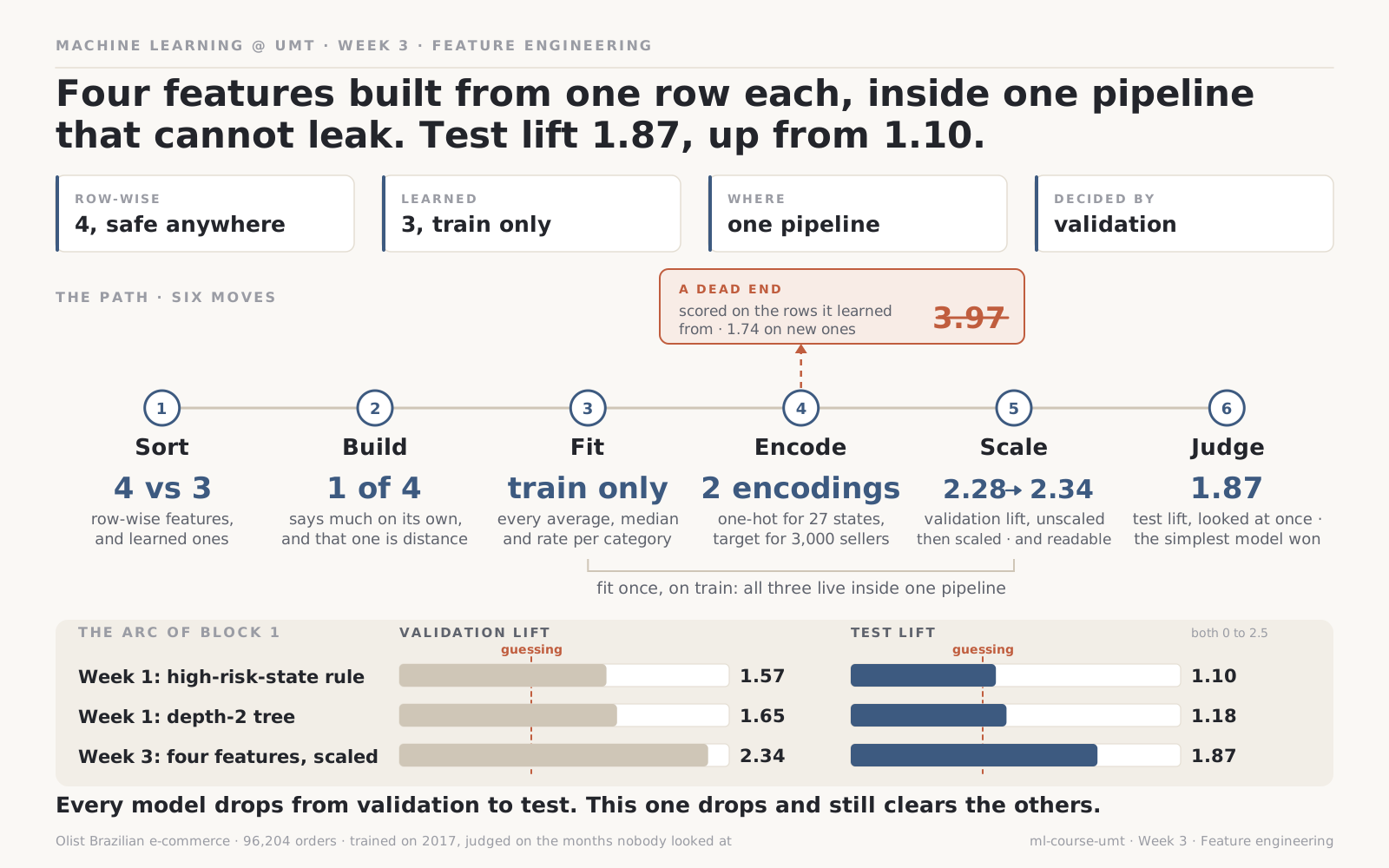
The same frame, filled in. The scoreboard is Block 1's whole arc: the same three models, on validation and on the future.

Features come in two kinds. Row-wise features, built from one row, are safe anywhere. Learned features, built from many rows, must be learned from training rows only, and a statistic computed over the whole dataset is the quietest leak there is. The transformer pattern, fit to learn and transform to apply, and the pipeline that holds every step together, make that rule hard to break by accident. Categories are encoded according to how many values they have, with cross-fitting for target encoding, and linear models are scaled so they train properly and can be read. Then each feature earns its place on validation. Here the simplest features won, and the model they built held up once on the future: a test lift of 1.87, up from 1.10.

Next week asks what that number hides: at which threshold we should act, which orders the model gets wrong, and whether it fails some customers far more than others.

Next: Week 04 · Evaluation & error analysis

Resources

• scikit-learn, Pipelines and composite estimators. The official guide to Pipeline and ColumnTransformer.
• scikit-learn, Target Encoder. How cross-fitting works inside TargetEncoder.
• scikit-learn, Common pitfalls. Short, and almost entirely about the leaks in this page.
• scikit-learn cheatsheet on this site, for every pattern above in one place.

Quote

Learn from the past, apply to the present, and let validation decide what stays.