Calculus for ML
At a glance
You need this in: Week 06 (optimization), Week 07 (regularization), Week 12 (neural networks) Estimated time: 35 minutes Assumed: you have met derivatives before, even if you have forgotten the rules
In this course calculus has one job: explaining how a model learns its weights. The linear algebra page described a model that already had good weights. This page is about how it finds them.
The notation carries over directly. \(X\) is the data matrix, \(\mathbf{w}\) the weights, \(\hat{\mathbf{y}} = X\mathbf{w}\) the predictions.
1. A derivative is a slope, and a slope points downhill
Take a loss that depends on a single weight:
At \(w = 5\) the derivative is \(+4\): the loss rises as \(w\) grows, so move left. At \(w = 1\) it is \(-4\): the loss falls as \(w\) grows, so move right. At \(w = 3\) it is zero, and you have arrived.
That is gradient descent, before any notation. Look at the slope, step the other way, repeat.
2. The derivatives you actually need
Five, and that genuinely covers this course.
| Function | Derivative | Where it turns up |
|---|---|---|
| \(x^n\) | \(n x^{n-1}\) | Squared error |
| \(e^x\) | \(e^x\) | The sigmoid |
| \(\ln x\) | \(1/x\) | Log loss |
| \(\sigma(x) = \dfrac{1}{1+e^{-x}}\) | \(\sigma(x)\,\bigl(1 - \sigma(x)\bigr)\) | Logistic regression, neural networks |
| \(\lvert x \rvert\) | \(+1\) or \(-1\), undefined at 0 | Lasso, and the source of its quirks |
Plus two rules you use without noticing: the derivative of a sum is the sum of the derivatives, and constants come along for the ride.
3. Partial derivatives
A real model has many weights. A partial derivative asks how the loss changes when you nudge one weight and hold every other one still.
Same rules as before. Everything that is not the variable you are differentiating by is treated as a constant.
4. The gradient points uphill, so step against it
Collect every partial derivative into one vector and you have the gradient.
It points in the direction the loss increases fastest. So the update rule steps the opposite way:
The minus sign is the whole idea. \(\eta\) is the learning rate: how big a step to take.
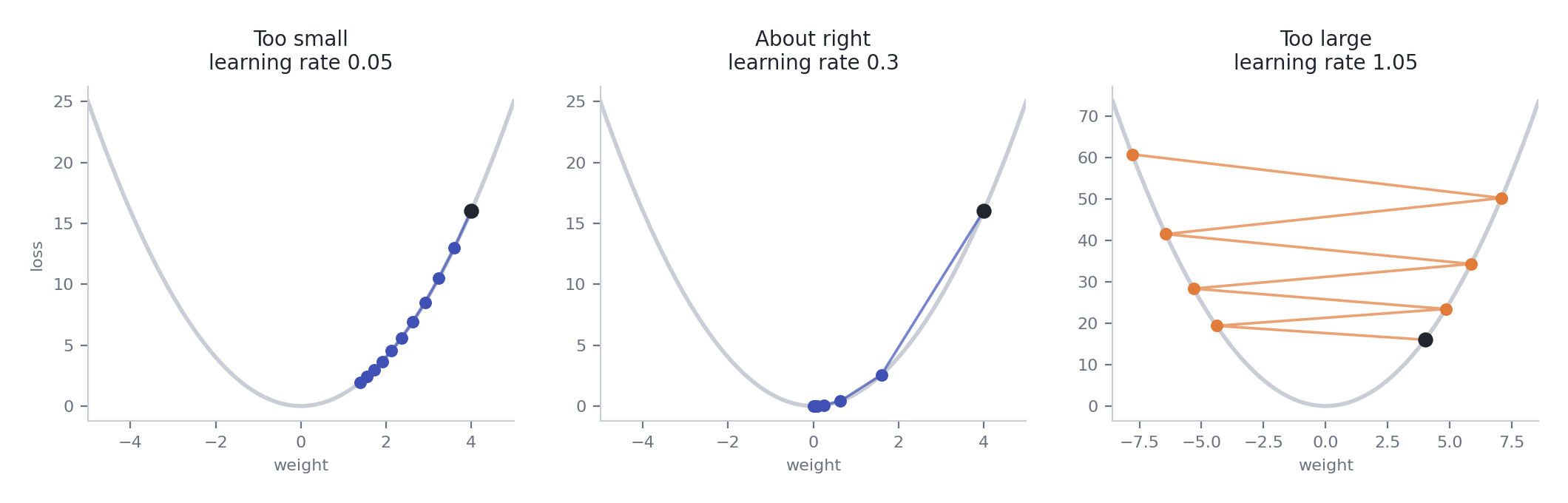
Same loss, same starting point, three step sizes. Too small crawls. Too large overshoots further every step and never arrives.
Where this lands
Week 6. When your gradient descent diverges in the lab, this figure is the first thing to check against. A loss that grows every iteration almost always means the learning rate is too large.
5. The gradient of mean squared error
This is the section that pays for the rest. The loss for linear regression is
Differentiate with respect to \(\mathbf{w}\). The inner term \(\mathbf{y} - X\mathbf{w}\) has derivative \(-X\), the square brings down a 2, and the transpose from the linear algebra page arranges the shapes:
Read it in words: the residuals \(\mathbf{y} - X\mathbf{w}\), weighted by each feature, averaged. Features that line up with large errors get large gradients.
And the code, which is the same line:
Check the shapes: X.T is (k, n), residual is (n,), so grad is (k,), the same shape as w. It has to be, since you subtract one from the other.
Where this lands
The Week 6 drill has you write exactly these three lines inside a loop. Derive it here once by hand, and the lab becomes typing something you understand rather than copying something you do not.
6. Adding a penalty
Regularization adds a term to the loss, so it adds a term to the gradient.
Ridge adds \(\lambda\lVert\mathbf{w}\rVert^2\), whose gradient is \(2\lambda\mathbf{w}\). The update becomes
Every step shrinks every weight by a fixed fraction before the usual update. That is why the same idea is called weight decay in neural networks.
Lasso adds \(\lambda\lVert\mathbf{w}\rVert_1\). The absolute value has no derivative at zero, so plain gradient descent does not apply cleanly, and solvers use other methods instead. The kink at zero is also exactly what lets lasso park weights at zero and leave them there.
Where this lands
Week 7. The linear algebra page explains the same difference through the shape of the two norms. This is the other half of the picture.
7. Log loss has the same shape
For logistic regression the predictions are probabilities, \(\mathbf{p} = \sigma(X\mathbf{w})\), and the loss is log loss:
Working through the derivative takes a page, and the sigmoid's derivative from section 2 cancels almost everything. What is left is
Compare it with section 5. Both are \(X^\top\) times prediction minus truth. Two different models, two different losses, one gradient pattern. This is not a coincidence, and it is part of why these two models are the base case for everything else.
8. Why feature scaling matters to the optimizer
Suppose one feature is area in square metres, somewhere between 30 and 300, and another is floor number, between 1 and 10. The gradient along the area weight is enormous compared with the one along floor.
A learning rate small enough to be stable for area is far too small to move floor at all. A learning rate large enough for floor makes area overshoot. The loss surface is a long narrow valley, and gradient descent bounces between its walls instead of travelling along it.
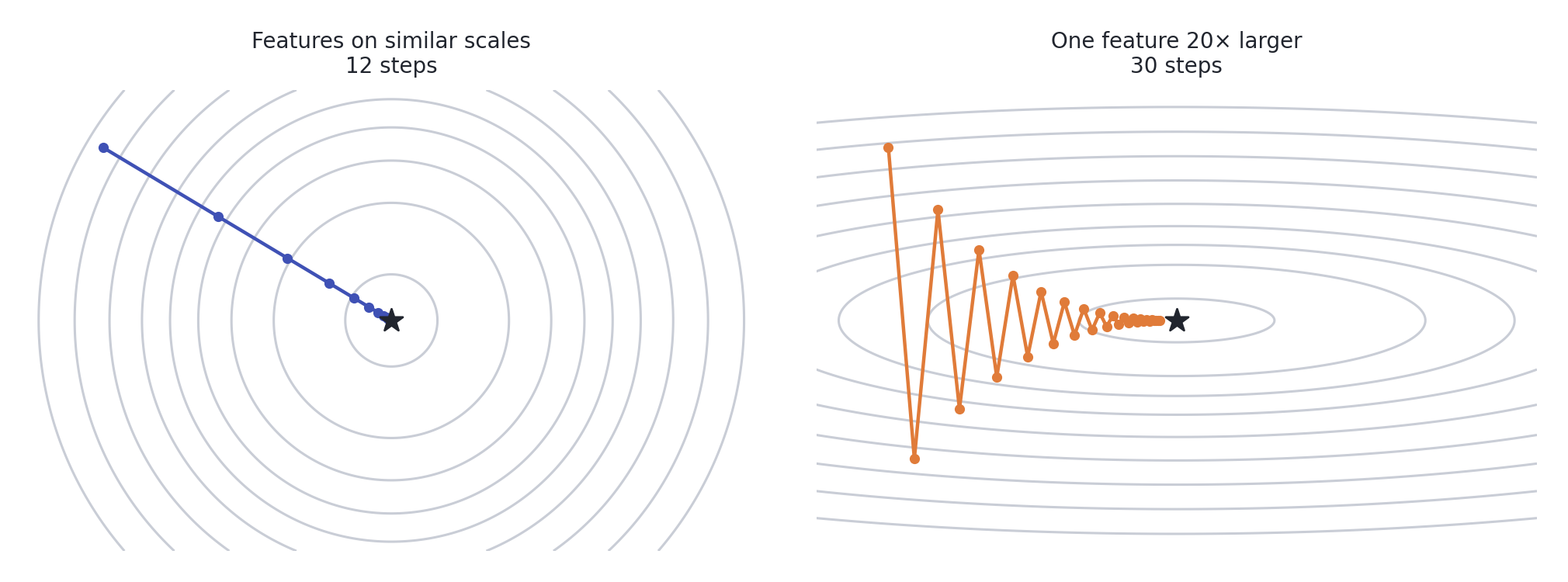
Both paths are real gradient descent runs. Left: comparable scales, straight to the minimum. Right: one feature twenty times larger, and the path zigzags across the valley.
from sklearn.preprocessing import StandardScaler

X_scaled = StandardScaler().fit_transform(X_train)   # fit on train only
Where this lands
Week 6, and this is the failure the lab is built around. You will run gradient descent on unscaled features, watch it zigzag or diverge, then scale and watch it converge. Tree models do not care about scaling. Anything trained by gradient descent cares a great deal.
9. Convexity
A convex loss has one minimum, and every downhill path leads there.
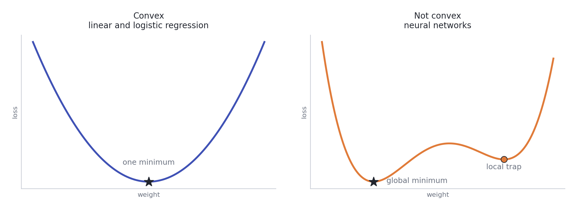
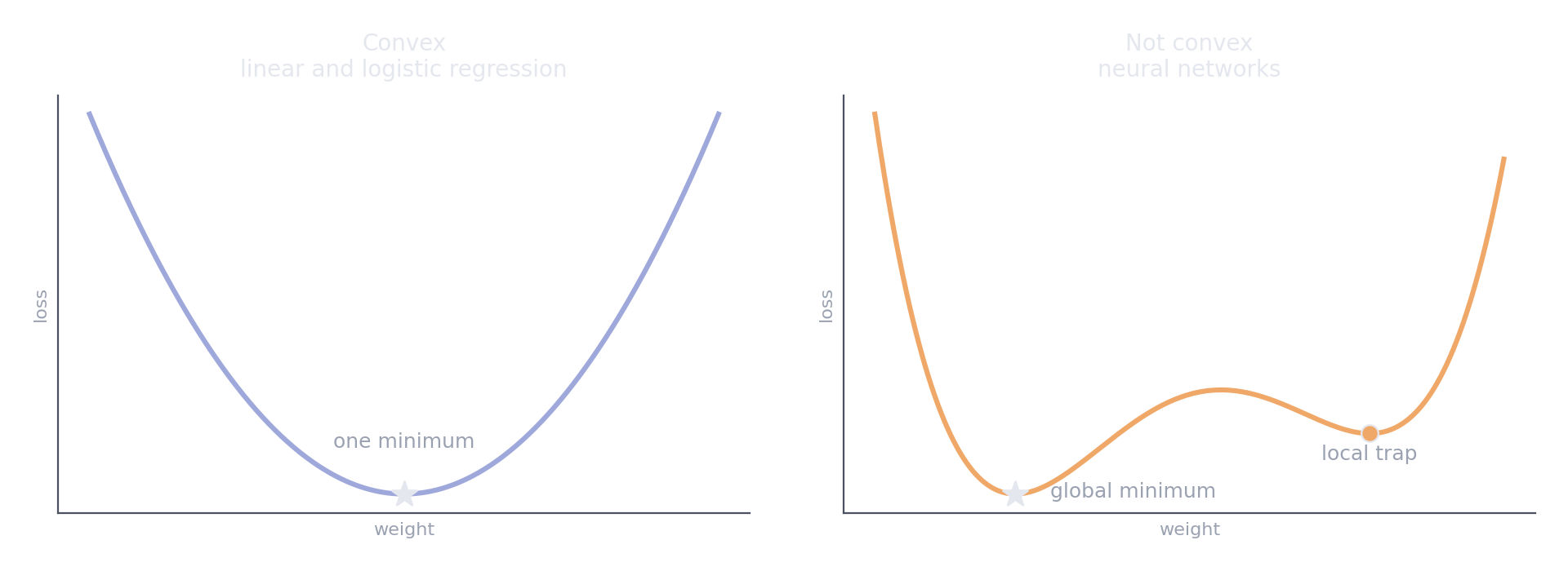
Left: one minimum, so where you start does not matter. Right: descent from the right-hand side settles in the local trap and stops.
Linear and logistic regression are convex, so gradient descent finds the best possible weights given enough steps. Neural networks are not, so the answer depends on where you start and on randomness during training. That is why deep learning results vary between runs, and why you set seeds.
10. The chain rule
When one thing depends on another which depends on another, the derivatives multiply.
In words: a change in \(x\) causes a change in \(g\), which causes a change in \(f\). Multiply the two sensitivities.
Logistic regression is already a chain: weights produce a score \(z = \mathbf{w}^\top\mathbf{x}\), the score becomes a probability \(p = \sigma(z)\), the probability produces a loss \(L\).
Where this lands
Week 12. A neural network is the same chain with more links. Backpropagation is this rule applied from the loss backwards, one layer at a time, reusing each product as it goes. There is no new idea in it, only more multiplication.
11. Check your gradient numerically
When your gradient descent refuses to converge, the first suspect is the gradient itself. Estimate each partial derivative by nudging one weight a tiny amount in both directions:
def numerical_grad(loss, w, eps=1e-6):
    grad = np.zeros_like(w)
    for i in range(len(w)):
        step = np.zeros_like(w)
        step[i] = eps
        grad[i] = (loss(w + step) - loss(w - step)) / (2 * eps)
    return grad

np.allclose(numerical_grad(loss, w), my_gradient(w), atol=1e-5)
If the two disagree, your derivative is wrong, and no amount of tuning the learning rate will fix it. This takes a minute to write and can save an evening.
What this page skips
Quick reference
| Concept | Formula |
|---|---|
| Update rule | \(\mathbf{w} \leftarrow \mathbf{w} - \eta\,\nabla L\) |
| MSE gradient | \(-\tfrac{2}{n}\, X^\top(\mathbf{y} - X\mathbf{w})\) |
| Log loss gradient | \(\tfrac{1}{n}\, X^\top(\mathbf{p} - \mathbf{y})\) |
| Ridge penalty gradient | \(2\lambda\mathbf{w}\) |
| Sigmoid derivative | \(\sigma(x)(1 - \sigma(x))\) |
| Chain rule | \((f \circ g)' = f'(g) \cdot g'\) |
| Symptom | Likely cause |
|---|---|
| Loss grows every step | Learning rate too large |
| Loss falls, but painfully slowly | Learning rate too small, or features not scaled |
| Loss zigzags | Features on very different scales |
| Loss never behaves, whatever the rate | Gradient is wrong. Check it numerically. |
Resources
- 3Blue1Brown, Essence of Calculus. The intuition behind derivatives and the chain rule, in short videos.
- Mathematics for Machine Learning, chapter 5. Free PDF, the full treatment of vector calculus.
- Why Momentum Really Works. An interactive article on why gradient descent zigzags and what momentum does about it. Read it after Week 6.
- Andrej Karpathy, micrograd. Backpropagation built from scratch in about a hundred lines. Ideal preparation for Week 12.
Next in this section: Probability and statistics, which is how you decide whether the model you trained is actually any good.