Recurrent Neural Networks

Recurrent Neural Networks (RNNs) are designed to handle sequential data: they allow a model to process information where the order matters (like sentences, stock prices, or sensor readings) by maintaining a "memory" of what has happened before.

They solve a fundamental limitation of Feed-Forward and Convolutional networks: Standard models assume every input is independent, which fails when the meaning of a word depends on the three words that preceded it.

From Spatial to Temporal (The "Why")

In CNNs, you analyzed spatial patterns: static snapshots where pixels relate to their neighbors. However, many real-world problems are temporal, meaning the data functions more like a "story" than a single picture.

1. Variable Length (Elasticity)

CNNs and standard networks require a fixed input size (e.g., 224x224 pixels). RNNs are "elastic"; because they process data in a loop, the same mathematical operation can handle a 3-word sentence or a 300-word paragraph.

2. Context & Order (Sequential Logic)

In temporal data, the order changes the meaning entirely.

• Context: In "The bank of the river," the word "river" tells the model that "bank" is land, not a building.
• Direction: The sequence \([1, 2, 3]\) (increasing) is fundamentally different from \([3, 2, 1]\) (decreasing), even though the "pixels" (numbers) are identical.

3. The Hidden State (\(h_t\))

RNNs maintain a hidden state, which acts as a running summary of the past. As each new input (\(x_t\)) arrives, the model combines it with the previous summary (\(h_{t-1}\)) to create a new one.

Key Applications: Where Order Matters

Field	Temporal Factor
NLP	Translation & Sentiment. Words only make sense within the context of a sentence.
Time-Series	Finance & Weather. Today’s value is a direct consequence of the historical trend.
Audio	Speech-to-Text. A sound wave is meaningless without the millisecond that preceded it.
Robotics	Trajectory Prediction. Predicting a pedestrian's path based on their last 5 steps.

Professional Takeaway: If the data has a "before" and an "after," it is a temporal problem. RNNs allow the model to track the "flow" rather than just the "frame."

RNN Architecture: The Essentials

What is an RNN?

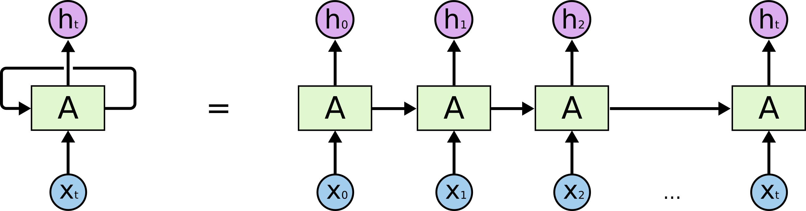
A Recurrent Neural Network (RNN) is a model designed for data that unfolds over time. Unlike standard feed-forward networks that process an entire input in one pass and then "forget" it, an RNN processes sequences element-by-element.

It utilizes a feedback loop where the output from one calculation is fed back into the next. This looping mechanism allows the model to maintain a continuous thread of information, making it possible for the network to understand that what happens at step 10 is directly influenced by what happened at step 1.

The Hidden State (Internal Memory)

The Hidden State (\(h_t\)) is the mathematical engine of this memory. It is a vector that serves as the "bridge" between time steps, carrying context forward. At every time step \(t\), the RNN performs a dual-input calculation:

1. The New Data (\(x_t\)): The specific information present at the current moment (e.g., the current word or stock price).
2. The Existing Memory (\(h_{t-1}\)): The summary of everything the model has learned from the beginning of the sequence up until the previous step.

The model combines these two inputs to produce a new hidden state (\(h_t\)). This isn't just a replacement; it is an update. The model weighs the new information against the old memory to decide how the "story" has changed. This updated \(h_t\) is then passed to the next step, ensuring the context is never lost.

Because the same weights are applied at every single step of the loop, the model learns "universal" rules for how to update its memory, regardless of where it is in the sequence.

Bidirectional RNNs (BRNN)

In many real-world scenarios, the "future" context is just as vital as the "past." A standard RNN is like reading a sentence one word at a time through a narrow slit; you don't know how the sentence ends until you get there. However, to correctly interpret a word, you often need to see what follows it.

A Bidirectional RNN solves this by using two independent hidden layers:

1. The Forward Pass: Processes the sequence from start to finish (time \(1 \to T\)).
2. The Backward Pass: Processes the sequence from end to start (time \(T \to 1\)).

The model then merges the information from both passes at every time step. This allows the network to have a "complete view" of the sequence.

Example in Translation: Consider the phrase: "The green apple..." vs. "The green light..." In some languages, the translation of "green" might change based on whether it describes a fruit or an object. A Bidirectional RNN knows that "apple" or "light" is coming, allowing it to make the correct decision for "green" immediately.

Professional Insight: BRNNs are the standard for tasks where the entire sequence is available at once (like text or recorded audio). They are not used for real-time applications where the future data hasn't happened yet (like live stock market trading).

The Gradient Crisis (The Bottleneck)

Standard RNNs struggle with long-term dependencies because of how they learn using calculus (Backpropagation Through Time). As the error signal travels backward from the end of a sequence to the beginning, it undergoes repeated multiplications that can make training unstable.

The Vanishing Gradient Problem

As the "signal" of the error is passed back through many time steps, it is repeatedly multiplied by the weights. If those weights are small (less than 1), the signal shrinks exponentially until it effectively disappears.

• The Result: The model "forgets" the beginning of long sequences and only learns from the most recent inputs.
• The "Why" (Example): Imagine a sentiment analysis model reading a 100-word product review that starts with "I originally hated this brand, but..." and ends with 90 words describing a recent great experience. Due to the vanishing gradient, the model may "forget" the initial context of the brand's history and only focus on the latest positive words.

The Exploding Gradient Problem

If the weights are large (greater than 1), the signal grows exponentially as it moves backward. The gradients become so massive that they cause the model's weights to update too drastically, leading to mathematical "breakdown" (often seen as NaN or Not-a-Number values in your code).

• The Result: The model becomes unstable and cannot converge on a solution because the "steps" it takes during learning are too large.
• The Solution (Gradient Clipping): We implement a safety cap. If the gradient exceeds a certain threshold, we scale it back down.
• The "Why" (Example): In the same review model, an exploding gradient might cause the model to see a single word like "disaster" and react so strongly that it completely overwrites all other learned patterns, ruining the model's overall accuracy in one training step.

Vanishing gradients are a structural problem (solved by LSTMs/GRUs), while exploding gradients are an optimization problem (solved by Gradient Clipping)..

Advanced Cells: LSTM & GRU (The Engine Upgrade)

Standard RNNs fail because they try to squeeze all past information into a single hidden state. To fix this "fading memory," researchers developed specialized architectures that use gates; mathematical filters that decide which information to keep, which to ignore, and which to pass forward.

LSTM (Long Short-Term Memory)

The LSTM solves the vanishing gradient problem by introducing a Cell State (\(C_t\)). Think of the Cell State as a high-speed "conveyor belt" that runs straight through the entire sequence with only minor linear interactions. This allows information to flow across hundreds of time steps without being heavily diluted.

To manage this conveyor belt, the LSTM uses three specialized gates:

1. Forget Gate: This is the first stop. It looks at the new input and the previous memory and decides what is no longer relevant.
   • Example: In a story, if a new character enters, the Forget Gate might "erase" the detailed physical description of a character who just left the scene.
2. Input Gate: This gate decides which parts of the new incoming data are worth storing in the Cell State.
   • Example: If the current word is a subject like "The Professor," the Input Gate recognizes this as vital context and records it onto the conveyor belt.
3. Output Gate: Finally, this gate decides what the model should actually "show" at the current step. It filters the long-term Cell State to produce the short-term Hidden State (\(h_t\)).
   • Example: Even if the memory knows the character's full biography, the Output Gate ensures the model only focuses on the character's current action for the next prediction.

GRU (Gated Recurrent Unit)

The GRU is a streamlined, more modern alternative to the LSTM. It simplifies the architecture by merging the Cell State and Hidden State into a single vector.

Instead of three gates, it uses two:

1. Update Gate: A combination of the "Forget" and "Input" functions—it decides how much of the past to keep and how much new information to add simultaneously.
2. Reset Gate: Determines how much of the past memory to ignore when calculating a new candidate memory.

Because GRUs have fewer parameters, they are faster to train and less prone to overfitting on smaller datasets. However, LSTMs remain the gold standard for long, complex sequences where a strict separation between long-term and short-term memory is required.

Rule of thumb: LSTMs are generally more powerful for very complex data, while GRUs are faster to train and often perform just as well on smaller datasets.

How to do it by hand (Worked mini-example)

Manual RNN State Update

Let’s look at how a simple RNN updates its "memory." Imagine a sequence of numbers. At step \(t\), we have:

• Input (\(x_t\)): 0.5
• Previous Hidden State (\(h_{t-1}\)): 0.1
• Weights (\(W\)): 0.8 (Weight for input) and 0.5 (Weight for hidden state)

Formula (Simplified): \(h_t = \text{activation}( (x_t \times W_{in}) + (h_{t-1} \times W_{hid}) )\)

1. Multiply input: \(0.5 \times 0.8 = 0.4\)
2. Multiply previous memory: \(0.1 \times 0.5 = 0.05\)
3. Sum them: \(0.4 + 0.05 = 0.45\)
4. Apply activation (e.g., Tanh): \(\tanh(0.45) \approx 0.42\)

New Memory (\(h_t\)): 0.42. This value is now passed to the next step.

Real-World Utility: Where Order Matters

While CNNs are the gold standard for static images, RNN-based architectures (especially LSTMs and GRUs) are the workhorses for streaming or sequential data. If your task involves "predicting the next step" or "summarizing a history," these are your primary tools.

• Natural Language Processing (NLP): Used for translation and sentiment analysis. Unlike a CNN that sees words as isolated features, an RNN understands that the meaning of a word depends on the words that came before it.
• Time-Series & Finance: Essential for stock market prediction or energy grid load forecasting. RNNs detect trends (rising/falling) over time that a standard feed-forward network would miss.
• Signal Processing: Used in heart rate monitoring (ECG) or speech recognition. The model treats the audio or sensor wave as a continuous sequence rather than a single block of data.

Keras Snippets + Industry Best Practices

Implementing RNNs, LSTMs, and GRUs

In Keras, switching between these architectures is as simple as changing the layer name. Note the use of Bidirectional, which allows the model to look at both past and future context simultaneously.

from tensorflow import keras
from tensorflow.keras import layers

model = keras.Sequential([
    # A Bidirectional LSTM: Processes the sequence forward and backward
    # return_sequences=True is required because the next layer is also an RNN
    layers.Bidirectional(layers.LSTM(64, return_sequences=True), input_shape=(20, 1)),

    # A standard GRU layer: Often faster to train than LSTM
    # return_sequences=False because the next layer is a Dense layer (we only need the final summary)
    layers.GRU(32, return_sequences=False),

    layers.Dense(1)
])

Key Parameters to Master:

• return_sequences=True: The layer outputs the hidden state for every time step in the sequence. You must use this when "stacking" RNNs so the next layer has a full sequence to read.
• return_sequences=False (Default): The layer only outputs the final hidden state. Use this when you are finished with sequential processing and are ready to transition to a Dense layer for a final prediction.

Professional Tip: When working with very long sequences, even LSTMs can struggle. In those cases, the industry often turns to Attention mechanisms or Transformers, which we will cover in a later module.

Industry Orientations (Practical)

• Standardize your input: RNNs are very sensitive to the scale of data. Always use scaling (like Min-Max or Standard Scaling).
• Use LSTMs/GRUs by default: Almost never use SimpleRNN. The vanishing gradient problem makes it impractical for real-world tasks.
• Watch your sequence length: Very long sequences (e.g., >500 steps) can still be difficult for LSTMs. Consider breaking them into smaller chunks.

Standardize or Normalize Input

RNNs use activation functions like \(\tanh\) and sigmoid repeatedly across time steps. If your data isn't scaled, the math can "saturate," meaning the model stops learning. Always scale your features to a range like \([0, 1]\) or \([-1, 1]\).

from sklearn.preprocessing import MinMaxScaler
scaler = MinMaxScaler(feature_range=(0, 1))
# Reshape and scale your sequential data before feeding to the model
scaled_data = scaler.fit_transform(raw_data)

Use LSTMs/GRUs by Default

The SimpleRNN is essentially a legacy layer for modern tasks. Because it cannot effectively carry information over long gaps, industry practice is to start with LSTM or GRU.

# Avoid: layers.SimpleRNN(32)
# Standard: 
model.add(layers.LSTM(64, activation='tanh')) 
# Or for faster training:
model.add(layers.GRU(64))

Manage Sequence Length

Processing extremely long sequences (e.g., thousands of steps) makes the memory "conveyor belt" less effective. It is often better to slice your data into smaller, manageable windows.

# Instead of one sequence of 1000 steps, use windows of 50
# X_train shape: (samples, window_size, features)
def create_windows(data, window_size=50):
    # Logic to slide a window across the timeline
    ...

Implementation of Gradient Clipping

To prevent the "Exploding Gradient" problem where weight updates become too large and "break" the model (NaN errors), always cap the gradients in your optimizer.

from tensorflow.keras.optimizers import Adam
# clipnorm ensures the gradient vector does not exceed a certain magnitude
opt = Adam(learning_rate=0.001, clipnorm=1.0)
model.compile(optimizer=opt, loss='mse')

Quick Glossary

• Timestep: A single point in a sequence (e.g., one word in a sentence or one day in a stock chart).
• Hidden State (\(h\)): The model's "short-term" memory that changes at every step to represent the current context.
• Cell State (\(C\)): The "long-term" memory found only in LSTMs; it acts as a protected highway for information to travel across many steps.
• Gating: The mechanism of using mathematical filters to "block" or "allow" specific information to pass into the model's memory.
• BPTT (Backpropagation Through Time): The specific way we train RNNs by "unrolling" the loops into a long chain so we can apply standard calculus.
• Many-to-Many / Many-to-One: Terms describing the input/output flow. For example, "Many-to-One" takes a whole sentence and outputs a single sentiment score (Positive/Negative).
• Gradient Clipping: A safety technique that caps the size of gradients during training to prevent the "Exploding Gradient" problem.
• Sequence Padding: The process of adding zeros to shorter sequences so that all inputs in a batch have the same length for the model to process.

REMEMBER: RNNs allow models to understand the "story" of the data, rather than just seeing a single snapshot.