Object Detection with YOLO

Introduction

Image classification answers a simple question: what is in this image?
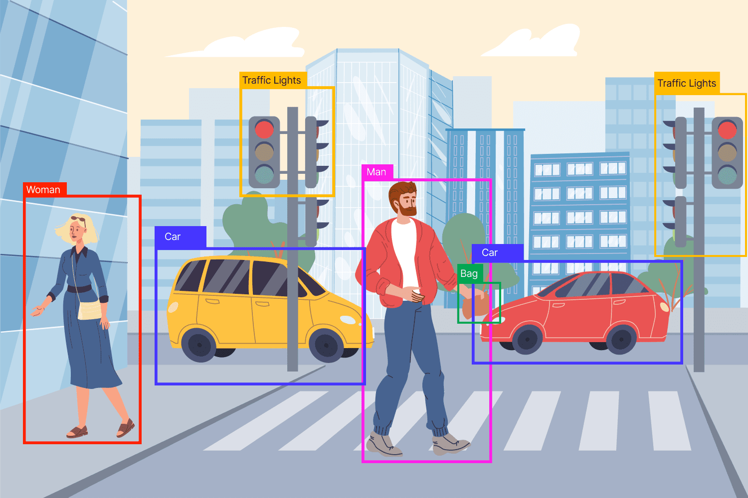
Object detection answers a harder one: what objects are in this image, and where are they?

That means object detection must do two jobs at once:

• Classify each object, such as person, car, dog, or bicycle
• Localize each object by drawing a bounding box around it

This makes object detection much more challenging than image classification.
Instead of giving one label for a full image, the model must find multiple objects, separate them from the background, and place boxes in the correct locations.

From Classification to Detection

Before studying YOLO, it helps to separate three related tasks.

Image Classification

In image classification, the model looks at the whole image and predicts one main label.

Example:

• A photo of a dog → dog
• A photo of a car → car

This is the simplest task because the model does not need to say where the object is.

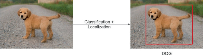
Localization

Localization adds one more job.
The model must predict:

• What the object is
• Where it is

So instead of only saying “dog,” it also draws a bounding box around the dog.

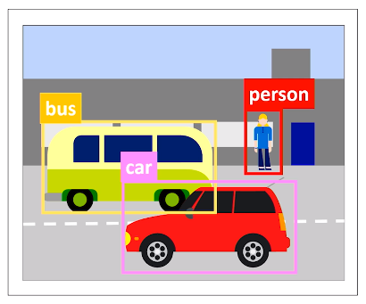
Object Detection

Object detection goes one step further.
Now the image may contain many objects, and the model must detect all of them.

Example:

• One image may contain a dog, a bicycle, and two people
• The model must output four bounding boxes
• Each box must have a class label and a confidence score

This is why object detection is harder:

• There may be multiple objects
• Objects can overlap
• Objects can be small or large
• Some objects may appear only partly in the image
• The background may be cluttered

A good mental model is this:

• Classification = What is here?
• Localization = What is here, and where?
• Detection = What objects are here, where are they, and how many are there?

What is Object Detection?

Object detection is the task of finding objects in an image and predicting a bounding box and class label for each one.

A typical object detector outputs something like this:

• Box 1: person, 0.96 confidence
• Box 2: dog, 0.91 confidence
• Box 3: bicycle, 0.88 confidence

Each prediction usually contains:

• A bounding box
• A class label
• A confidence score

What is a Bounding Box?

A bounding box is a rectangle that surrounds an object.

It tells the model where the object is located.
Boxes are commonly represented in one of two ways:

• Corner format: \((x_1, y_1, x_2, y_2)\)
• Center format: \((x, y, w, h)\)

Where:

• \(x, y\) = box center
• \(w\) = width
• \(h\) = height

The goal is not just to classify correctly, but to place the box as accurately as possible.

The Old Approach: Sliding Windows

Before modern detectors like YOLO became popular, one common approach was the sliding windows algorithm.

What is the Sliding Windows Algorithm?

The idea is simple:

1. Take a small window
2. Place it over one part of the image
3. Run a classifier on that window
4. Move the window slightly
5. Repeat across the whole image

The classifier asks at each step:

• “Does this small region contain an object?”
• “If yes, what object is it?”

This process is repeated many times over many parts of the image.

Why Sliding Windows Makes Sense

This approach is intuitive because it turns detection into many small classification problems.

Instead of asking the model to understand the whole image at once, we ask:

• Does this patch contain a dog?
• Does this patch contain a car?
• Does this patch contain a person?

That idea is conceptually easy to understand, which is why it is a good learning starting point.

The Main Problem

Sliding windows is very slow.

Why?

Because the model must check:

• Many positions
• Many window sizes
• Many aspect ratios

For one image, that can mean thousands of separate classifications.

Why Multiple Sizes Are Needed

Objects do not all appear at the same scale.

• A nearby car may be large
• A far-away car may be tiny

So one fixed-size window is not enough.
You need many windows of different sizes.

That increases the computation even more.

Main Weaknesses of Sliding Windows

• Too slow for real-time use
• Repeats similar computations again and again
• Struggles with different object sizes efficiently
• Produces many overlapping candidate boxes
• Becomes expensive as images get larger

Why It Still Matters

You should learn sliding windows because it explains the motivation behind modern object detection.

It helps answer an important question:

Why did researchers want a new approach like YOLO?

Because they wanted a detector that could look at the image once instead of thousands of times.

The Big Shift: Single-Shot Detectors

Modern object detection became much faster when models stopped treating detection as thousands of separate classification problems.

What is a Single-Shot Detector?

A single-shot detector predicts object locations and class labels in one forward pass through the network.

That means the model looks at the image once and directly outputs:

• Bounding boxes
• Confidence scores
• Class predictions

This is very different from the sliding windows idea.

Why “Single-Shot” Matters

The phrase “single-shot” means detection happens in one main pass rather than through many repeated searches.

This creates major advantages:

• Much faster inference
• Better fit for real-time applications
• More efficient use of shared image features

Instead of separately analyzing every patch, the network learns the whole detection task end to end.

Why This Leads to YOLO

YOLO is one of the best-known single-shot detectors.

Its name stands for:

You Only Look Once

That name captures the core idea perfectly:

• Do not scan the image piece by piece
• Do not run thousands of mini-classifications
• Look once, predict everything

What is the YOLO Algorithm?

YOLO is an object detection algorithm that predicts bounding boxes and class probabilities directly from the image in one pass.

The Core Idea

YOLO treats object detection as a single learning problem.

Instead of splitting the task into many separate steps, it trains one model to learn:

• Where objects are
• Whether an object exists
• What class each object belongs to

This makes YOLO simple in concept and powerful in practice.

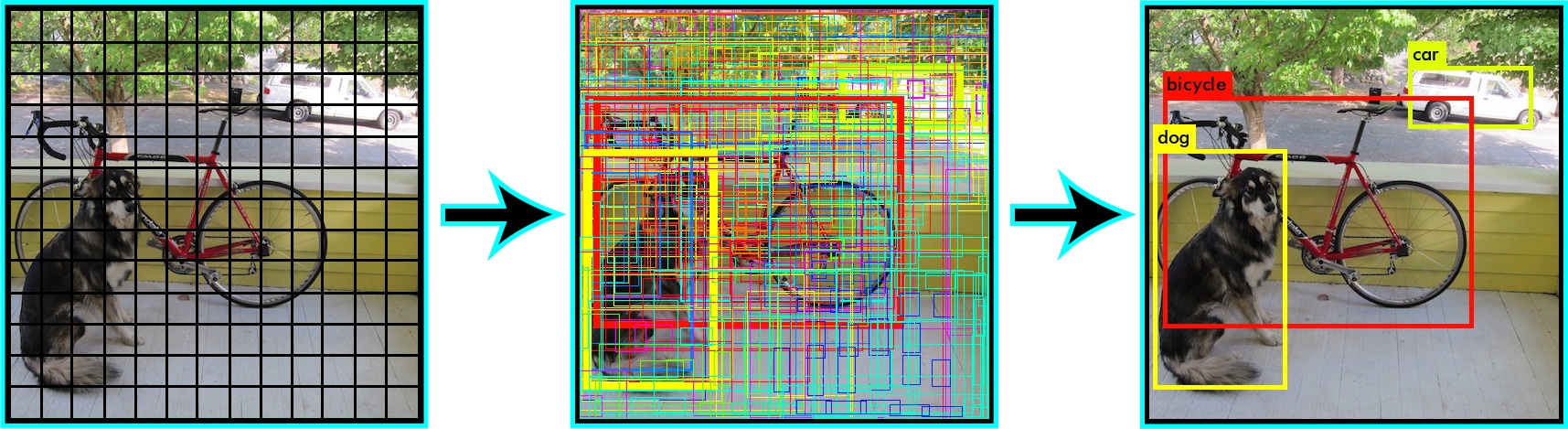
The Grid Idea

A beginner-friendly way to understand classic YOLO is this:

• Divide the image into a grid
• Each grid cell becomes responsible for detecting objects whose center falls inside it
• Each cell predicts one or more bounding boxes
• Each predicted box includes a confidence score and class information

This helps the model organize predictions across the image.

What YOLO Predicts

For each candidate object, YOLO typically predicts:

• Box position
• Box size
• Objectness score
• Class probabilities

Let’s break that down.

1. Box Position

The model predicts where the object is located.

2. Box Size

The model predicts how wide and tall the object is.

3. Objectness Score

This answers:

• “Is there really an object here?”
• “How confident is the model that this box contains something meaningful?”

4. Class Probabilities

If an object is present, the model predicts what it is:

• person
• dog
• car
• bicycle
• and so on

Why YOLO Is Fast

YOLO is fast because the network shares computation across the entire image.

Instead of repeatedly analyzing overlapping regions, it processes the image once and reuses learned visual features to make all predictions together.

That makes YOLO especially useful in applications like:

• Self-driving systems
• Security cameras
• Robotics
• Sports analytics
• Mobile vision apps

The Main Tradeoff

YOLO gains speed by making strong, direct predictions.

Historically, this sometimes meant a tradeoff:

• Extremely fast detection
• But more difficulty with very small objects or crowded scenes

That tradeoff has improved a lot across newer YOLO versions, but the core learning idea stays the same.

How YOLO Makes Predictions

Step 1: The Image Enters the Network

The full image is sent into a convolutional neural network.

The network extracts visual features such as:

• Edges
• Shapes
• Textures
• Patterns

These features help the model recognize objects.

Step 2: The Model Predicts Candidate Boxes

The detector predicts many possible boxes across the image.

Each candidate box usually includes:

• Position
• Size
• Objectness
• Class scores

At this stage, there may be many candidate boxes for the same object.

Step 3: Low-Confidence Predictions Are Removed

Predictions with very low confidence are usually filtered out first.

This reduces noise and keeps only boxes that seem meaningful.

Step 4: Overlapping Predictions Are Cleaned Up

Many boxes may point to the same object.

So the detector applies non-max suppression to remove duplicates.

Step 5: Final Detections Remain

The final result is a smaller set of predictions:

• One box per object, ideally
• A class label
• A confidence score

This makes the output readable and useful.

IoU: Intersection over Union

IoU is one of the most important ideas in object detection.

What Is IoU?

IoU stands for Intersection over Union.

It measures how much two bounding boxes overlap.

Usually, those two boxes are:

• The predicted box
• The ground-truth box (the correct answer from the labeled dataset)

Why IoU Matters

A predicted box may classify the right object but still be badly placed.

IoU helps answer:

How well does the predicted box match the true box?

A higher IoU means better overlap.

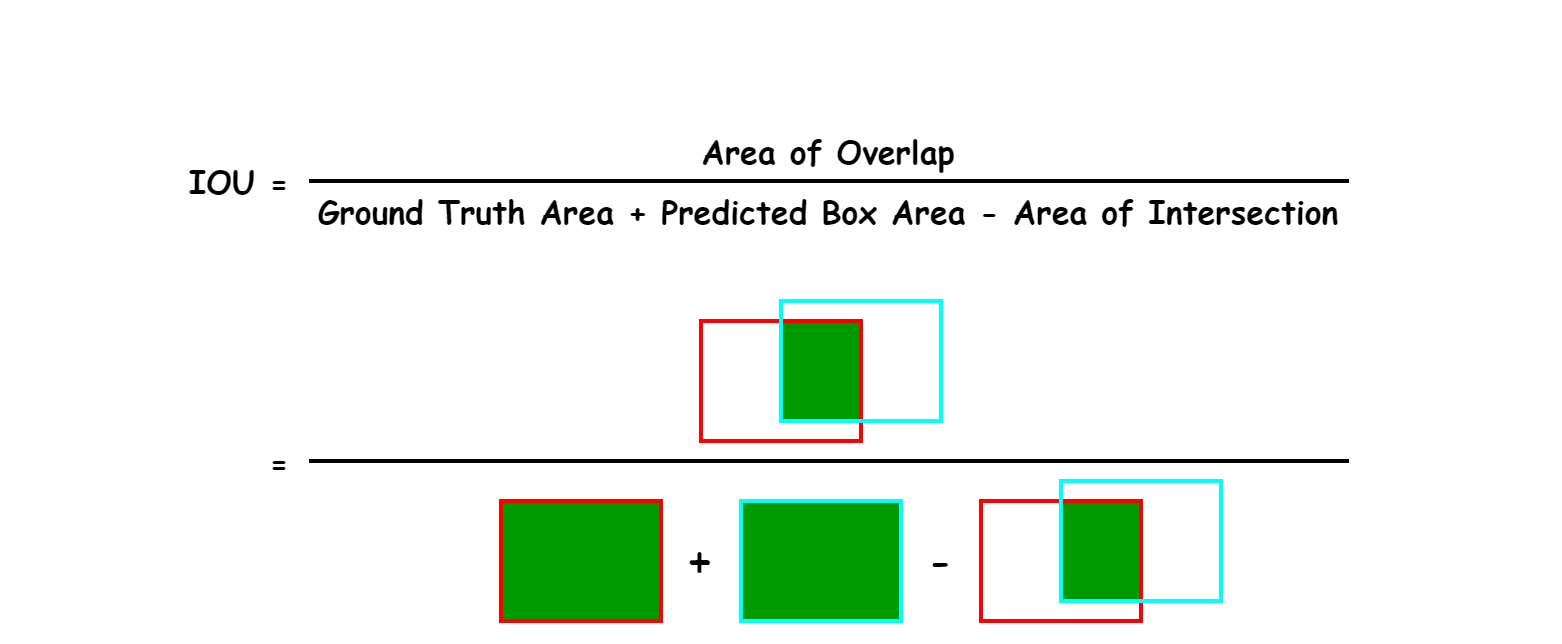
How Do You Calculate IoU?

IoU is defined as:

\[ IoU = \frac{\text{Area of Overlap}}{\text{Area of Union}} \]

Where:

• Overlap = the shared area between the predicted box and the true box
• Union = total area covered by both boxes together

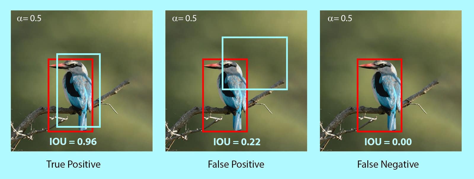
Intuition

• If two boxes do not overlap at all, IoU = 0
• If they overlap perfectly, IoU = 1
• If they overlap partly, IoU is somewhere between 0 and 1

Simple Example

Suppose:

• Predicted box area = 100
• Ground-truth box area = 120
• Overlap area = 80

Then:

\[ IoU = \frac{80}{100 + 120 - 80} = \frac{80}{140} \approx 0.57 \]

So the boxes overlap fairly well, but not perfectly.

Why IoU Is Used

IoU is used in at least two important ways:

• To decide whether a predicted box counts as correct
• To help remove duplicate predictions during non-max suppression

In many evaluation settings, a prediction is considered correct only if its IoU is above some threshold, such as 0.5.

What is Non-Max Suppression?

When a detector looks at an object, it often predicts several similar boxes around the same thing.

That creates duplicates.

The Problem

Imagine one dog in the image, but the model predicts:

• Box A with confidence 0.95
• Box B with confidence 0.91
• Box C with confidence 0.87

All three boxes overlap heavily and describe the same dog.

Without cleanup, the detector would appear to find three dogs instead of one.

What Non-Max Suppression Does

Non-max suppression, often called NMS, removes redundant boxes and keeps the best one.

The word “max” refers to keeping the box with the highest confidence.

How NMS Works

1. Start with all predicted boxes
2. Keep the box with the highest confidence
3. Compare it with the remaining boxes
4. Remove boxes whose IoU with it is too high
5. Repeat with the next highest-confidence box

Why IoU Appears Again

NMS uses IoU to decide whether two boxes are “too similar.”

If two boxes overlap a lot, they probably refer to the same object.

So NMS suppresses the weaker one.

Example

Suppose the top-scoring box has confidence 0.95.
If another box overlaps it with IoU 0.80, and the NMS threshold is 0.5, the second box is usually removed.

Why?

Because it is probably just a duplicate prediction of the same object.

Important Clarification

NMS does not improve a bad box.
It only filters overlapping predictions.

That distinction is important.

You may think NMS “fixes” detection quality.
It does not.

It simply chooses which predictions survive.

What Are Anchor Boxes?

Anchor boxes are a way to help the detector predict objects of different shapes and sizes.

Why They Are Needed

A single location in an image may need to describe different possible objects:

• A tall person
• A wide car
• A small dog
• A narrow bottle

If the model predicted only one generic box shape at each location, it would struggle to represent all these possibilities.

The Main Idea

Anchor boxes are predefined reference boxes.

They come in different:

• Widths
• Heights
• Aspect ratios

The model does not always predict a box completely from scratch.
Instead, it learns how to adjust these reference boxes to better match actual objects.

Intuition

Think of anchor boxes as starting templates.

For example, at one image location the model may consider:

• A tall narrow box
• A medium square box
• A wide short box

Then it learns which one best fits the object and how to shift or resize it.

Why Anchor Boxes Help

They make it easier to detect:

• Multiple objects from the same region
• Objects with different proportions
• Objects that appear at different scales

Common Pitfalls

Anchor boxes are not actual detections.
They are starting shapes used to guide prediction.

That is an important distinction.

How YOLO Uses Confidence

In object detection, confidence is not just “how sure the class is.”

Practicioners often confuse several different scores, so it helps to separate them.

Objectness Score

This score answers:

• Is there an object in this box?
• Or is this mostly background?

Class Probability

This score answers:

• If an object is present, what class is it?

Confidence in Practice

A final detection score often reflects both:

• Whether an object exists
• How likely the predicted class is

So a box with high class probability but low objectness may still not be trusted much.

This is why two boxes with the same label can still have different final scores.

How to Evaluate Object Detection

A detector is not judged only by whether it names objects correctly.

It must also place boxes accurately.

That is why object detection evaluation is more complex than simple classification accuracy.

Precision and Recall

Before mAP, you should know two basic ideas.

Precision

Precision asks:

Of all the boxes the model predicted as objects, how many were correct?

High precision means:

• Few false positives
• The model does not make many bad detections

Recall

Recall asks:

Of all the true objects in the image, how many did the model find?

High recall means:

• Few missed objects
• The model finds most of what is actually there

These two ideas often trade off against each other.

• A very cautious detector may have high precision but low recall
• A very aggressive detector may have high recall but lower precision

What is mAP?

mAP is the standard summary metric for object detection.

It is one of the most important evaluation concepts to understand.

What Does mAP Mean?

mAP stands for mean Average Precision.

Let’s separate the parts.

• Precision tells how many predicted detections are correct
• Average Precision (AP) summarizes precision across different recall levels for one class
• mAP is the mean of AP values across classes

So mAP gives one overall number that reflects detection quality across the dataset.

Why mAP Is Better Than Plain Accuracy

Plain accuracy is not enough for object detection because:

• There may be multiple objects per image
• Bounding box quality matters
• Confidence thresholds matter
• Duplicate detections matter

mAP captures this more realistically.

High-Level Process for Calculating mAP

A begineer-friendly version is:

1. Choose a class, such as “dog”
2. Collect all predicted dog boxes from the dataset
3. Sort them by confidence score
4. Match predictions to ground-truth boxes
5. Decide whether each prediction is a true positive or false positive using an IoU threshold
6. Build a precision-recall curve
7. Compute the area under that curve = AP for that class
8. Repeat for all classes
9. Average the AP values = mAP

How IoU Is Used in mAP

A prediction is usually counted as correct only if:

• The class is correct
• The IoU with a ground-truth box is above a threshold

For example:

• mAP@0.5 means a prediction counts as correct if IoU \(\geq 0.5\)
• A stricter evaluation may require higher overlap

AP vs mAP

This is a common source of confusion.

• AP = one class
• mAP = average across classes

Example:

• AP for person = 0.82
• AP for dog = 0.76
• AP for bicycle = 0.70

Then mAP is the average of those values.

What About mAP@0.5:0.95?

Some benchmarks report mAP over multiple IoU thresholds, often from 0.5 to 0.95.

This is stricter than only using 0.5.

Why?

Because the detector must perform well not only at loose overlap thresholds, but also at tighter ones.

That rewards more accurate localization.

How the Core Ideas Connect

At this point, the major concepts should fit together like one system.

• Object detection finds objects and their locations
• Sliding windows is the older, slower way to do this
• Single-shot detectors make predictions in one pass
• YOLO is a famous single-shot detector
• IoU measures how well boxes overlap
• Non-max suppression removes duplicate boxes
• Anchor boxes help model different shapes and sizes
• mAP measures overall detection performance

This is the big picture:

1. The model predicts many boxes
2. Confidence scores rank those boxes
3. IoU helps judge overlap quality
4. NMS removes duplicates
5. mAP evaluates how well the full system performs

Common Pitfalls

These are the mistakes practicioners make most often.

1. Confusing Classification with Detection

Classification predicts one label for an image.
Detection predicts many boxes plus labels.

2. Thinking IoU Measures Confidence

It does not.
IoU measures overlap between boxes.

3. Thinking NMS Improves Prediction Quality

It does not fix bad boxes.
It only removes redundant ones.

4. Thinking Anchor Boxes Are Final Objects

They are just reference shapes used during prediction.

5. Ignoring Box Location During Evaluation

A detector can guess the right class and still be wrong if the box is badly placed.

6. Confusing AP with mAP

AP is for one class.
mAP is averaged over classes.

7. Believing YOLO Is Only About Speed

YOLO is famous for speed, but the deeper idea is unified end-to-end detection in one model.

Intuition Recap

A good way to remember the topic is this:

• Sliding windows: search everywhere, many times
• Single-shot detection: predict everything together
• YOLO: one network, one pass, many predictions
• IoU: how well boxes overlap
• NMS: remove duplicate boxes
• Anchor boxes: starting shapes for flexible predictions
• mAP: the main score for detection quality

If you understand these seven ideas clearly, you already have a strong foundation in object detection.

Final Learning Checklist

You should be able to explain each of these after reading:

• What object detection is
• Why it is harder than classification
• How sliding windows works
• Why sliding windows is slow
• What a single-shot detector is
• Why YOLO is fast
• What YOLO predicts
• How IoU is computed
• Why non-max suppression is necessary
• What anchor boxes do
• What mAP measures

That is the conceptual foundation needed before moving on to training pipelines, loss functions, datasets, or implementation details.