Deep Learning Architectures

2014-2017 changed everything. Three papers showed we could build networks 100x deeper:

• Inception (Szegedy et al., Google, 2015): 22 layers, compute-efficient
• ResNet (He et al., 2016): 152 layers, skip connections
• DenseNet (Huang et al., Cornell, 2017): every layer talks to every layer

These papers didn't just win competitions; they showed new ways to connect layers to build deeper, more efficient, and more powerful neural networks.

This tutorial breaks down their key ideas + shows the Keras code to use them instantly.

📋 Table of Contents

1. The Problem
   Why deep networks historically failed

2. Foundational Enablers
   What made deep learning possible (ReLU, BatchNorm, initialization)

3. Case Study 1: Inception
   "Going deeper with convolutions" (Szegedy et al., Google, CVPR 2015)

4. Case Study 2: ResNet
   "Deep Residual Learning for Image Recognition" (He et al., CVPR 2016)

5. Case Study 3: DenseNet
   "Densely Connected Convolutional Networks" (Huang et al., Cornell, CVPR 2017)

6. Architecture Decision Matrix
   When to use what + Keras applications

7. Key Takeaways
   Evolution of connection design

1. The Problem: Why Deep Networks Failed

Deep networks (50+ layers) wouldn't train reliably. Gradients—the learning signal—disappeared or exploded.

How gradients flow back (backpropagation)

• Prediction error → loss
• Loss flows backward through chain rule: each layer's gradient = previous gradient × local derivative.
• 50-100 layers means 50-100 multiplications.

Vanishing gradients (signal → 0)

• Sigmoid/tanh derivatives are ~0.25 or less.
• Multiply 50 times: \(0.25^{50} \approx 10^{-35}\) (vanished).
• Result: Early layers don't update. Loss plateaus flat.

Exploding gradients (signal → ∞)

• Weights > 1 multiply: \(1.1^{50} \approx 130\), \(1.1^{100} \approx 13,780\).
• Result: Wild updates → oscillating/NaN loss.

Key insight: Deeper networks should learn better features. But couldn't train reliably before 2015.

2. Foundational Enablers

Before 2014, deep networks couldn't train reliably. Three simple ideas changed that and paved the way for Inception, ResNet, and DenseNet.

ReLU Activation: Fixed vanishing gradients

ReLU solved the core problem with sigmoid/tanh activations. Instead of derivatives shrinking to near-zero, ReLU's derivative is exactly 1 (when x > 0).

• ReLU(x) = max(0, x) — simple and fast
• No saturation: gradients flow cleanly through layers
• Tradeoff: "Dying ReLUs" (neurons output 0 forever), fixed by variants later

Weight Initialization: Kept signal balanced

Random initialization often caused gradients to explode or vanish immediately. Xavier/He initialization scales weights so variance stays roughly constant across layers.

• Xavier: variance = 2/(fan_in + fan_out) (good for sigmoid/tanh)
• He: variance = 2/fan_in (perfect for ReLU, accounts for zeroing)
• Result: Every layer gets reasonable gradients from the start

Batch Normalization: Stabilized training entirely

BatchNorm normalizes each layer's inputs to have mean=0, std=1 (computed over mini-batch). This prevents "internal covariate shift" where layer inputs drift during training.

• How: BN(x) = γ*(x - μ)/σ + β (learnable scale/shift)
• Why: Smoother gradients + higher learning rates possible
• Bonus: Built-in regularization effect (less overfitting)
• Keras: layers.BatchNormalization() after conv/dense layers

Impact: Suddenly 20-50 layer networks trained reliably. Architecture papers could focus on connections instead of fighting optimization.

3. Case Study 1: Inception

"Going deeper with convolutions" (Szegedy et al., Google, CVPR 2015)

The Big Picture: Depth vs Compute Explosion

Problem: More layers means much more computation. A simple 22-layer network uses 100x more processing power than AlexNet.

Stacking layers naively explodes compute costs. Inception found a smarter way.

Core insight: Use parallel convolutions at different scales, then concatenate. This captures multi-scale features efficiently.

Result: GoogLeNet = 22 layers, 5M parameters (vs AlexNet's 60M), won ImageNet 2014.

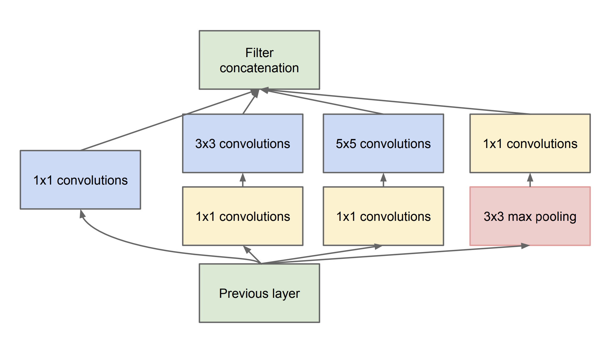
Key Innovation: Inception Module

Big idea: Instead of picking one filter size, Inception runs all sizes at once (1×1, 3×3, 5×5, pooling), then combines everything.

Why it's brilliant:

• 1×1 filters: fine details (edges, corners)
• 3×3 filters: textures and shapes
• 5×5 filters: larger objects/patterns
• Pooling: handles objects at different scales

The cost-saver: 1×1 convolutions shrink channels first.

192 channels × 5×5 conv = 4,800 operations/pixel
1×1 first (192→16) × 5×5 = 1,280 operations/pixel
**74% cheaper!**

Result: Much richer features + way less computation.

Breakdown:

• 1×1 conv: Dimension reduction (cheap)
• Parallel paths: 1×1, 3×3, 5×5, pool (multi-scale features)
• Concat: Richer representation than single conv

Full GoogLeNet Architecture

Imagine you're designing a network and you want it deep but not expensive. GoogLeNet stacks 9 Inception modules in a very clever way.

First, they replace the giant final layer that everyone used. Instead of flattening 7×7×1024 features into millions of parameters, they use global average pooling. This shrinks the spatial size to 1×1 while keeping all the rich features—zero extra parameters!

Second, they add two auxiliary classifiers in the middle. Think of your network as a tall building. Gradients sometimes struggle to climb back up from the top to the early floors. These middle classifiers give gradients "shortcuts" so early layers keep learning.

Third, they carefully downsample between Inception blocks (224→28→14→7 pixels). Each stage focuses on different scales naturally.

The numbers speak for themselves:

• 22 layers deep (most before were 8-11)
• 5 million parameters (vs VGG's 138 million)
• Won ImageNet 2014 with 6.67% top-5 error

In Keras, you get the evolved version instantly:

from tensorflow.keras.applications import InceptionV3
model = InceptionV3(weights='imagenet')

The genius: Inception modules gave them depth. Smart design choices made it practical.

Lesson: Parallel multi-scale convolutions + 1×1 dimension reduction = depth without compute explosion.

4. Case Study 2: ResNet

"Deep Residual Learning for Image Recognition" (He et al., CVPR 2016)

Imagine you're stacking more layers expecting better accuracy. Past 20 layers, accuracy drops. The deeper network performs worse than a shallower one.

The shocking discovery: This wasn't an optimization problem. Deeper networks were forgetting what shallower networks already learned. They degraded.

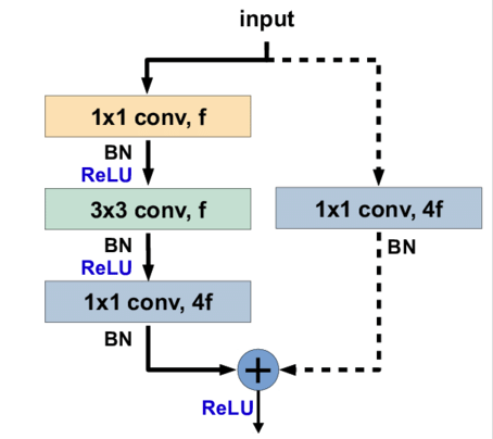
The beautiful solution: Don't make layers learn the complete transformation from input to output. Instead, teach them just the difference (residual): output = input + layers(input).

Why Skip Connections Work

Think of gradients flowing backward through 100 layers. Each layer multiplies the gradient by its derivative. Multiply 100 times by numbers < 1 = gradient ≈ 0.

Skip connections guarantee flow: gradient = normal_path_gradient + 1. That "+1" from the identity path ensures gradients always reach early layers.

Two block designs:

• Basic block: Two 3×3 convolutions + skip (ResNet-18/34)
• Bottleneck block: 1×1→3×3→1×1 + skip (ResNet-50/101/152)

The Complete Architecture

How ResNet Is Organized

The network starts with a stem—a simple 7×7 convolution followed by a pooling step. This first stage takes the raw input image and distills the most basic shapes, edges, and textures, while also shrinking the image size so the later layers can work more efficiently.

After the stem, the network moves into four main stages, each built from many small computational units called residual blocks. Each stage has three characteristics:

1. It applies several of these residual blocks in sequence, all working at the same image size.
2. At the start of the stage, the image size is reduced by about half, typically by using a slightly larger step in the computations.
3. At the same time, the number of internal “feature channels” is doubled, so the network becomes richer in detail and more expressive.

For example:

• In Stage 1, three residual blocks process an image that is about 56×56 in size, using 256 internal channels.
• In Stage 2, four blocks work on a 28×28 image with 512 channels.
• In Stage 3, six blocks handle a 14×14 image with 1024 channels.
• In Stage 4, three blocks take the 7×7 image with 2048 channels.

After these four stages, the network performs a simple averaging step across the remaining small grid, which summarizes all the learned information into a fixed‑length vector. This vector is then mapped to predictions across 1000 different classes.

The results were astonishing. A plain 20‑layer network without these special connections had about 7.0% error, while the 34‑layer ResNet cut that error to about 3.6%. More dramatically, the 152‑layer version—over four times deeper—achieved roughly the same 3.6% error, proving that the extra depth was not wasted.

In practice, you can load a pre‑trained ResNet in Keras with just one line:

from tensorflow.keras.applications import ResNet50
model = ResNet50(weights='imagenet')

In short, the key insight of ResNet is that deeper networks can actually learn better, as long as the information and gradients can flow smoothly from the beginning of the network all the way to the end.

5. Case Study 3: DenseNet

"Densely Connected Convolutional Networks" (Huang et al., CVPR 2017)

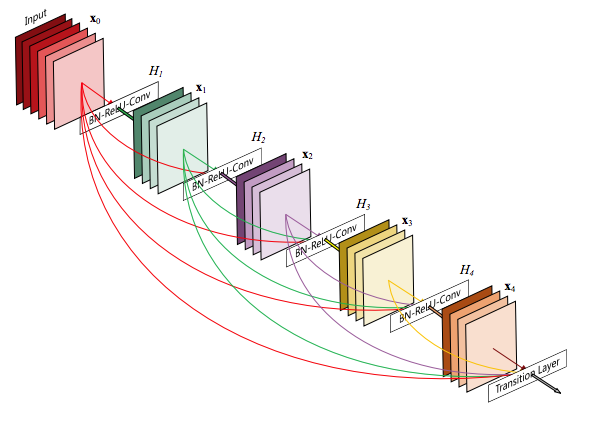
In traditional networks, each layer typically receives information only from the immediately preceding layer. DenseNet changes this pattern fundamentally: every layer receives feature maps from all previous layers in the same dense block, and each layer passes its own feature maps forward to all subsequent layers.

This means that the input to layer \(k\) is a concatenation of the outputs from layers \(1, 2, \dots, k-1\), plus its own computations. Instead of forcing each layer to relearn features that earlier layers have already captured, DenseNet lets it directly build on them, encouraging strong feature reuse and smoother gradient flow throughout the network.

Why Dense Connections Help

As the network processes an image, early layers capture simple patterns such as edges and textures. Middle layers combine these into more complex structures like shapes and object parts. Later layers assemble these structures into full object representations.

The key idea in DenseNet is that there is no need for each new layer to recompute features that earlier layers have already learned. Instead, each layer can directly reuse the feature maps computed by all previous layers, allowing information to accumulate and be shared efficiently across the network.

Each layer:

• Takes a concatenated stack of all previous feature maps
• Adds 1×1 convolutions to keep sizes manageable
• Returns new feature maps back to the stack

The Architecture Pattern

DenseNet starts with a stem (7×7 conv + pool), then builds the network from dense blocks separated by transition layers.

Each dense block:

• 6–12 layers (depending on depth)
• Each layer has 4×growth_rate channels added
• Typical growth_rate = 32 (doubles channels every 8 layers)

Transition layers:

• 1×1 conv to reduce channels
• 2×2 pool to halve spatial size
• Remove 50% of previous features

Why Dense Connections Work So Well

DenseNet’s dense connectivity pattern brings three main advantages:

1. Extreme feature reuse: Each layer receives the feature maps from all earlier layers in the same block, so it can combine information from many different levels of abstraction rather than relying only on the immediately preceding layer. This encourages richer representations and smoother learning.

2. Strong implicit regularization: The many cross‑layer connections distribute gradients more evenly and make it harder for the network to overfit to any single pathway. In effect, the architecture behaves as if it has built‑in regularization, improving generalization.

3. Compact models: Because features are reused rather than recomputed, the network can achieve high accuracy with relatively fewer parameters. This leads to smaller model sizes and faster inference while maintaining competitive performance.

Keras (immediately available):

from tensorflow.keras.applications import DenseNet121
model = DenseNet121(weights='imagenet')

Bottom line: DenseNet proved that dense feature reuse outperforms traditional residual connections for many tasks.

6. Architecture Decision Matrix

When to use what and how to load them in Keras

Choosing the right architecture depends on your task, data size, and hardware constraints. Here is a practical guide to decide which backbone to use and how to load it via Keras applications.

When to use ResNet

Use ResNet when:

• You want a solid, well‑tested baseline for image classification, object detection, or segmentation.
• You care about good performance with moderate depth and stable training.
• You are working with moderate GPU memory (ResNet‑50, 101, 152 are widely supported).

In Keras, you can load ready‑made ResNet models with pretrained ImageNet weights like this:

from tensorflow.keras.applications import ResNet50, ResNet101, ResNet152

model_50  = ResNet50(  weights='imagenet')
model_101 = ResNet101( weights='imagenet')
model_152 = ResNet152( weights='imagenet')

When to use DenseNet

Use DenseNet when:

• You want strong feature reuse and compact models.
• You care about high accuracy with relatively fewer parameters.
• You want an architecture that naturally encourages regularization and smoother gradient flow.

DenseNet is often a good choice when you want a rich representation without needing the largest models.

Keras applications:

from tensorflow.keras.applications import DenseNet121, DenseNet169, DenseNet201

model_121 = DenseNet121( weights='imagenet')
model_169 = DenseNet169( weights='imagenet')
model_201 = DenseNet201( weights='imagenet')

Quick decision table

Situation	Recommended backbone
General baseline, stable training	ResNet‑50
High accuracy, deeper model	ResNet‑101 or 152
Compact model, strong feature reuse	DenseNet‑121 or 201
ImageNet‑based transfer learning	Any of the above
Limited GPU memory	ResNet‑50 or DenseNet‑121

In practice, starting with ResNet‑50 or DenseNet‑121 is usually a safe choice. You can then experiment with deeper variants once you know your data size and hardware constraints.

7. Key Takeaways

Evolution of connection design

Over the past decade, the way we connect layers in deep networks has evolved from simple sequential chains into rich, structured connection patterns. These changes are not just cosmetic; they directly shape how information and gradients flow through the network, and thus how well the model learns.

Plain chains and the rise of residual connections

Early CNNs stacked layers in a strict pipeline: each layer only saw the output of the one before it. We now know that this simple chain limits both depth and stability. The introduction of ResNet’s skip (residual) connections changed this: each layer can freely combine its own computation with the signal from earlier layers. This made it possible to train networks that are much deeper while still preserving useful information from the input.

From residual to dense connectivity

DenseNet pushed the idea further. Instead of skipping only one or a few layers, every layer in a dense block receives feature maps from all previous layers. This dense pattern encourages strong feature reuse and spreads gradients across many paths, improving both accuracy and generalization. As a result, models can achieve high performance with fewer parameters and more compact storage.

What this evolution means in practice

• Connections are not just wiring; they are part of the model’s inductive bias.
• Deeper networks only work well when the architecture makes it easy for information and gradients to propagate.
• Modern architectures (ResNet, DenseNet, and their descendants) all share the same core lesson: design connectivity so that earlier information can reach later layers, and later gradients can reach earlier layers.

In short, the evolution of connection design has moved from simple chains to structured, reusable pathways. This shift is one of the main reasons modern deep networks can be both deep and effective.

The art of deep learning is not just in adding more layers, but in designing how they talk to each other.