Probability & Statistics for Machine Learning

This tutorial introduces probability and statistics fundamentals that are essential for understanding and applying machine learning. You'll learn to quantify uncertainty, understand distributions, and learn how probabilistic thinking enables ML models to make predictions under uncertainty.

Estimated time: 70 minutes

Why This Matters

Problem statement: Machine learning models don't make perfectly accurate predictions—they work with noisy, incomplete data and must quantify uncertainty. Without probability theory, we cannot model randomness, evaluate model reliability, or understand why algorithms make certain predictions.

Practical benefits: Probability provides the mathematical framework for handling uncertainty. Understanding distributions helps you choose appropriate models, compute confidence intervals, detect outliers, and interpret what predictions actually mean. Statistics enables you to validate model improvements and make data-driven decisions backed by evidence.

Professional context: Every ML algorithm involves probability. Classification models output probability distributions over classes ("80% cat, 20% dog"), regression models have probabilistic error terms, and neural networks learn probability distributions. Understanding these foundations is essential for building and trusting ML systems.

Prerequisites & Learning Objectives

Required knowledge: - Basic algebra and arithmetic - Understanding of functions and graphs - Familiarity with summation notation - Basic Python (minimal needed)

Learning outcomes: - Understand what probability measures and how to compute it - Distinguish between independent and disjoint events - Apply addition and multiplication rules for probabilities - Work with probability distributions and density functions - Compute and interpret mean, variance, and standard deviation - Recognize common distributions and their ML applications

Core Concepts

What is Probability?

Probability is a number between 0 and 1 that measures the likelihood of an event occurring.

Properties:

• \[0 \leq P(A) \leq 1$$ for any event $$A\]
• \[P(\text{certain event}) = 1\]
• \[P(\text{impossible event}) = 0\]

Example: Rolling a fair die

• \[P(\text{rolling a 6}) = \frac{1}{6} \approx 0.167\]
• \[P(\text{rolling even number}) = \frac{3}{6} = 0.5\]
• \(\(P(\text{rolling 7}) = 0\)\) (impossible)

In ML, probability models uncertainty. A classifier doesn't say "this IS a cat"—it says "I'm 85% confident this is a cat."

Random Variables

A random variable is a variable whose value is determined by chance.

Types:

• Discrete: Countable values (coin flips, dice rolls, number of customers)
• Continuous: Any value in a range (height, temperature, prediction error)

Features are random variables (customer age varies), predictions have uncertainty, and errors are random.

Basic Probability Notation

Key notation:

• \(\(P(A)\)\): Probability event \(\(A\)\) occurs
• \(\(P(A \cap B)\)\): Probability both \(\(A\)\) AND \(\(B\)\) occur
• \(\(P(A \cup B)\)\): Probability \(\(A\)\) OR \(\(B\)\) occurs
• \(\(P(A|B)\)\): Probability of \(\(A\)\) given \(\(B\)\) occurred (conditional)
• \(\(P(A^c)\)\): Probability \(\(A\)\) does NOT occur (complement)

Complement rule:

\[ P(A^c) = 1 - P(A) \]

Example: Weather forecasting

• \[P(\text{rain}) = 0.3\]
• \[P(\text{no rain}) = 1 - 0.3 = 0.7\]

Independent vs Disjoint Events

These concepts are different and often confused.

Disjoint (Mutually Exclusive): Cannot both happen simultaneously

• Rolling a 3 AND rolling a 5 on one die (impossible)
• \(\(A \cap B = \emptyset\)\) (empty)
• If \(\(A\)\) happens, \(\(B\)\) definitely doesn't

Independent: One event doesn't affect the other's probability

• Flipping two different coins
• \[P(A \cap B) = P(A) \cdot P(B)\]
• Knowing \(\(A\)\) occurred doesn't change \(\(P(B)\)\)

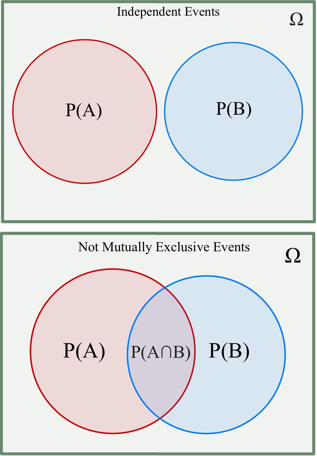
Critical distinction: Disjoint events are NEVER independent (unless probability is 0). If events can't occur together, they're dependent!

Naive Bayes (a ML model) assumes features are independent. Checking this assumption matters for model accuracy.

Addition Rule

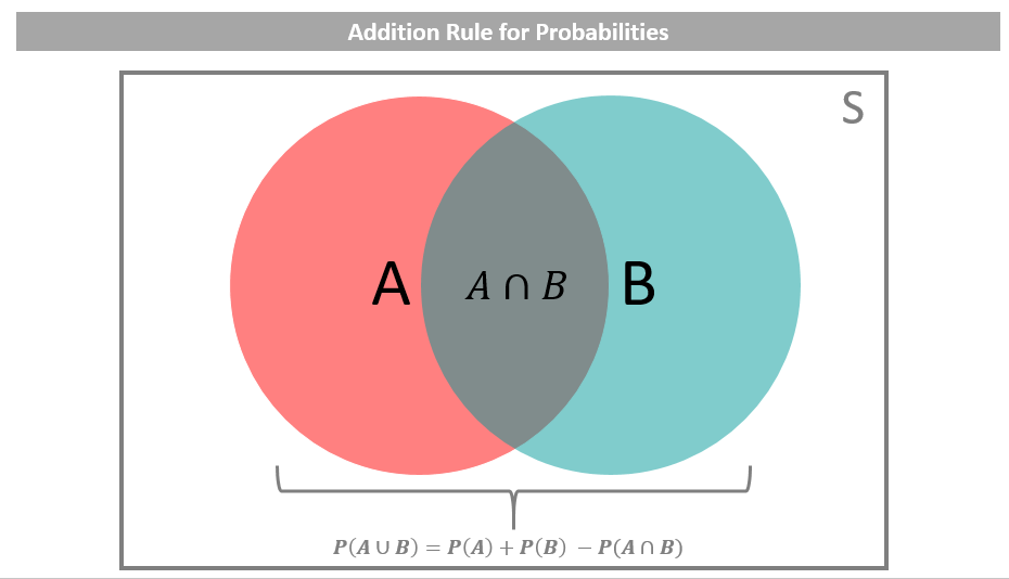
Computes probability that at least one event occurs.

General addition rule: $$ P(A \cup B) = P(A) + P(B) - P(A \cap B) $$

Why subtract? Adding \(\(P(A) + P(B)\)\) double-counts the overlap.

Special case (disjoint): $$ P(A \cup B) = P(A) + P(B) $$

Example: Drawing a card

• \[P(\text{Heart}) = \frac{13}{52} = 0.25\]
• \[P(\text{Ace}) = \frac{4}{52} = 0.077\]
• \[P(\text{Ace of Hearts}) = \frac{1}{52} = 0.019\]
• \[P(\text{Heart OR Ace}) = 0.25 + 0.077 - 0.019 = 0.308\]

Multiplication Rule

Computes probability that both events occur.

General multiplication rule: $$ P(A \cap B) = P(A) \cdot P(B|A) $$

Independent events: $$ P(A \cap B) = P(A) \cdot P(B) $$

Example: Drawing two cards without replacement

• \[P(\text{first ace}) = \frac{4}{52}\]
• \[P(\text{second ace | first ace}) = \frac{3}{51}\]
• \[P(\text{both aces}) = \frac{4}{52} \times \frac{3}{51} = 0.0045\]

ML connection: Computing joint probabilities in probabilistic models.

Conditional Probability and Bayes' Theorem

Conditional probability: Probability of \(\(A\)\) given \(\(B\)\) occurred

\[ P(A|B) = \frac{P(A \cap B)}{P(B)} \]

Bayes' Theorem (fundamental for ML): $$ P(A|B) = \frac{P(B|A) \cdot P(A)}{P(B)} $$

Example: Medical testing

• Disease prevalence: \(\(P(\text{disease}) = 0.01\)\) (1%)
• Test accuracy: \(\(P(\text{positive | disease}) = 0.95\)\)
• False positive rate: \(\(P(\text{positive | no disease}) = 0.05\)\)

Even with a positive test, the actual probability of having the disease is only about 16% because the disease is rare!

ML connection: Classification uses Bayes' theorem to compute \(\(P(\text{class | features})\)\) from \(\(P(\text{features | class})\)\).

Probability Distributions

A probability distribution describes how probability is allocated across possible values.

Types:

• Discrete: Probability Mass Function (PMF) - specific values have probabilities
• Continuous: Probability Density Function (PDF) - probabilities over ranges

All probabilities sum (discrete) or integrate (continuous) to 1.

Example: Fair die has uniform distribution

• \[P(X = 1) = P(X = 2) = \cdots = P(X = 6) = \frac{1}{6}\]

Probability Mass Function (PMF)

For discrete variables, PMF gives \(\(P(X = x)\)\) for each value.

Properties: - \(\(p_X(x) \geq 0\)\) for all \(\(x\)\) - \(\(\sum_x p_X(x) = 1\)\)

Example: Number of heads in 3 coin flips

Heads (x)	0	1	2	3
P(X = x)	1/8	3/8	3/8	1/8

Classification outputs are PMFs over classes.

Probability Density Function (PDF)

For continuous variables, PDF \(\(f(x)\)\) describes relative likelihood.

Key difference: For continuous variables, \(\(P(X = x) = 0\)\) for any specific \(\(x\)\). We compute probabilities over intervals:

\[ P(a \leq X \leq b) = \int_a^b f(x) \, dx \]

Properties:

• \[f(x) \geq 0\]
• \[\int_{-\infty}^{\infty} f(x) \, dx = 1\]
• Height \(\(f(x)\)\) is NOT a probability (can exceed 1)

Regression assumes errors follow a PDF (usually Gaussian/normal distribution).

Cumulative Distribution Function (CDF)

The CDF gives probability that a random variable is less than or equal to a value:

\[ F(x) = P(X \leq x) \]

Properties:

• \[0 \leq F(x) \leq 1\]
• \(\(F(x)\)\) is non-decreasing
• \[F(-\infty) = 0$$, $$F(\infty) = 1\]

Use: Compute probability over range $$ P(a < X \leq b) = F(b) - F(a) $$

Example: For standard normal distribution

• \(\(F(0) = 0.5\)\) (50% of values below 0)
• \(\(F(1) = 0.841\)\) (84.1% of values below 1)
• \(\(P(-1 \leq X \leq 1) = F(1) - F(-1) = 0.683\)\) (68.3%)

Percentiles

The p-th percentile is the value below which p% of observations fall.

Common percentiles:

• 25th (Q1), 50th (median), 75th (Q3)
• Interquartile Range: \(\(IQR = Q3 - Q1\)\)

Outlier detection: Values outside \(\([Q1 - 1.5 \times IQR, Q3 + 1.5 \times IQR]\)\)

ML connection: "This model's 90th percentile error is 5 units" means 90% of predictions have error ≤ 5.

Mean, Variance, and Standard Deviation

Let's use a simple dataset to illustrate: Test scores: 70, 75, 80, 85, 90

Mean (average): $$ \mu = \frac{70 + 75 + 80 + 85 + 90}{5} = \frac{400}{5} = 80 $$

The mean is the "center" or typical value.

Variance (spread): $$ \sigma^2 = \frac{(70-80)^2 + (75-80)^2 + (80-80)^2 + (85-80)^2 + (90-80)^2}{5} $$ $$ = \frac{100 + 25 + 0 + 25 + 100}{5} = \frac{250}{5} = 50 $$

Variance measures average squared distance from mean.

Standard deviation: $$ \sigma = \sqrt{50} \approx 7.07 $$

Standard deviation is typical distance from mean, in original units.

Interpretation: Most scores are within ±7 points of the average (80).

Properties:

• Higher variance/std dev = more spread out data
• Zero variance = all values identical
• Units: variance is squared, std dev matches data units

ML connection:

• Mean Squared Error (MSE) is the variance of prediction errors
• Standard deviation tells you typical prediction error magnitude
• Models try to minimize variance of errors

Common Probability Distributions

Uniform Distribution

Intuition: All values equally likely in a range.

Use cases:

• Random initialization of neural network weights
• Generating test data
• Modeling "no prior knowledge" scenarios

Example: Roll a fair die - each number has probability 1/6

ML application: Dropout in neural networks randomly selects neurons uniformly.

Normal (Gaussian) Distribution

Intuition: Bell-shaped curve, most values near the mean, symmetric.

Use cases:

• Natural measurements (height, IQ)
• Modeling errors and noise
• Central Limit Theorem applications

Parameters: Mean \(\(\mu\)\), variance \(\(\sigma^2\)\)

68-95-99.7 rule:

• 68% of data within 1 standard deviation of mean
• 95% within 2 standard deviations
• 99.7% within 3 standard deviations

ML applications:

• Linear regression assumes normal error distribution
• Gaussian Naive Bayes classifier
• Gaussian Processes
• Many algorithms assume normality for mathematical convenience

Bernoulli Distribution

Intuition: Single yes/no trial (success/failure).

Use cases:

• Coin flip (heads/tails)
• Binary classification (cat/not cat)
• Click/no click on ad

Parameters: \(\(p\)\) = probability of success

ML connection: Logistic regression outputs Bernoulli probabilities for binary classification.

Binomial Distribution

Intuition: Number of successes in \(\(n\)\) independent yes/no trials.

Use cases:

• Number of heads in 10 coin flips
• Number of customers who buy product
• Number of correct answers on multiple-choice test

Parameters: \(\(n\)\) (trials), \(\(p\)\) (success probability)

Mean: \(\(np\)\), Variance: \(\(np(1-p)\)\)

Example: Flip coin 10 times, expect 5 heads on average if fair.

Poisson Distribution

Intuition: Number of events occurring in fixed time/space interval when events happen independently at constant average rate.

Use cases:

• Number of emails received per hour
• Customer arrivals at store per day
• Website visits per minute
• Rare events

Parameters: \(\(\lambda\)\) (average rate)

ML connection: Poisson regression for count data (predicting number of occurrences).

Exponential Distribution

Intuition: Time between events in a Poisson process.

Use cases: - Time until next customer arrives - Lifetime of electronic component - Time between failures

Parameters: \(\(\lambda\)\) (rate)

Relationship: If events follow Poisson, time between events follows exponential.

Quick Reference

Concept	Definition	ML Application
Probability	Likelihood measure, 0 to 1	Quantifying uncertainty
Independent	\(\(P(A \cap B) = P(A)P(B)\)\)	Naive Bayes assumption
Addition rule	\(\(P(A \cup B) = P(A) + P(B) - P(A \cap B)\)\)	Multiple outcomes
Conditional	\(\(P(A\|B) = \frac{P(A \cap B)}{P(B)}\)\)	Context-dependent prediction
Bayes' theorem	\(\(P(A\|B) = \frac{P(B\|A)P(A)}{P(B)}\)\)	Classification
Mean	Center of distribution	Expected value
Variance	Spread measure	Error magnitude
Normal distribution	Bell curve	Error modeling
PMF	Discrete probabilities	Classification outputs
PDF	Continuous density	Regression errors
CDF	Cumulative probability	Percentiles, p-values

Summary & Next Steps

Key accomplishments: You've learned how probability quantifies uncertainty, mastered probability rules, understood distributions as models of randomness, computed statistical measures, and connected concepts to ML applications.

Best practices:

• Check distribution assumptions before applying methods
• Visualize data distributions to verify model fit
• Consider base rates (priors) in classification
• Use appropriate metrics for your distribution type

Connections to ML:

• Classification outputs probability distributions (softmax)
• Regression assumes error distributions (usually normal)
• Uncertainty quantification uses probability
• Bayesian ML treats parameters as random variables

External resources: - Khan Academy: Probability & Statistics - interactive lessons - 3Blue1Brown: Bayes' Theorem - visual explanation - Seeing Theory - visual introduction to probability