Introduction to Linear Algebra for Machine Learning
This tutorial introduces the fundamental concepts of linear algebra that form the mathematical foundation of machine learning. You'll build geometric intuition for vectors and matrices, understand key operations, and implement them in Python to solidify your understanding.
Estimated time: 60 minutes
Why This Matters
Problem statement: Machine learning algorithms operate on numerical data represented as vectors and matrices. Without understanding linear algebra fundamentals, it's impossible to grasp how models process data, optimize parameters, or make predictions.
Practical benefits: Linear algebra provides the mathematical framework to represent datasets, transform features, and understand model internals. Mastering these concepts enables you to implement ML algorithms from scratch, debug model behavior, optimize performance, and understand research papers describing new architectures.
Professional context: Every ML practitioner uses linear algebra daily. Linear regression uses matrix operations to find optimal coefficients, Principal Component Analysis (PCA) relies on eigenvalues for dimensionality reduction, Convolutional Neural Networks perform matrix multiplications and convolutions, and Support Vector Machines use linear algebra to find optimal decision boundaries.

Core Concepts
What is Linear Algebra?
Linear algebra is the branch of mathematics dealing with vectors, vector spaces, and linear transformations. It provides the language and tools to work with multidimensional data and transformations.
Why "linear"? Linear algebra studies operations that preserve vector addition and scalar multiplication. These operations can be visualized as transformations that keep grid lines parallel and evenly spaced.
Key insight: Every ML model learns a transformation from input space to output space. Linear algebra gives us the tools to understand and manipulate these transformations.
Key Terminology
Before learning about operations, let's establish essential vocabulary:
Scalar: A single number (e.g., 5, -3.14, 0.5)
Vector: An ordered collection of numbers representing magnitude and direction. Can be thought of as
- An arrow in space (geometric view)
- A list of coordinates (computer science view)
- A point in
n-dimensional space (mathematical view)
Matrix: A rectangular array of numbers arranged in rows and columns. Represents:
- A linear transformation (e.g., rotation, scaling, shearing)
- A collection of vectors (each row or column is a vector)
- A dataset (
rows = samples,columns = features)
Dimension: The number of components in a vector, or the size of the space it lives in
Linear transformation: An operation that transforms vectors while preserving lines and the origin
Step-by-Step Instructions
1. Understanding Vectors
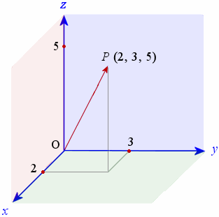
A vector is the fundamental building block of linear algebra. Think of it as an arrow pointing from the origin to a specific point in space.
Three perspectives on vectors:
Physics perspective: A vector has magnitude (length) and direction. For example, velocity or force.
Computer Science perspective: A vector is simply an ordered list of numbers: [1][2][3][4][5].
Mathematics perspective: A vector represents a point in n-dimensional space, where each number is a coordinate along one axis.
Why vectors matter in ML: Every data point is a vector. A customer's age, income, and purchase history form a 3D vector. An image with 1000 pixels is a 1000-dimensional vector.
Create a vector in Python:
# Create a 5-dimensional vector
my_vector = [1, 2, 3, 4, 5]

# Print the vector
print(my_vector)
print(f"This vector has {len(my_vector)} dimensions")
Expected output:
2. Vector Operations
There are several key operations which can be done with vectors.
Vectors can be combined and scaled using fundamental operations that have geometric interpretations.
Vector Addition
Adding two vectors $\(\mathbf{v_1} + \mathbf{v_2}\)$ means adding corresponding components element-wise. Geometrically, place the tail of $\(\mathbf{v_2}\)$ at the head of $\(\mathbf{v_1}\)$.
Why it matters: Gradient descent updates parameters by adding the gradient vector (scaled) to the current parameter vector.

Implement vector addition:
def add_vectors(vec1, vec2):
    """
    Add two vectors element-wise.
    Returns None if vectors have different lengths.
    """
    if len(vec1) != len(vec2):
        print("Error: Vectors must have the same dimension")
        return None

    result = []
    for i in range(len(vec1)):
        result.append(vec1[i] + vec2[i])

    return result

# Example usage
v1 = [1, 2, 3]
v2 = [4, 5, 6]
result = add_vectors(v1, v2)
print(f"{v1} + {v2} = {result}")
Expected output:
Vector Subtraction
Subtracting $\(\mathbf{v_2}\)$ from $\(\mathbf{v_1}\)$ gives the vector pointing from $\(\mathbf{v_2}\)$ to $\(\mathbf{v_1}\)$.
def subtract_vectors(vec1, vec2):
    """Subtract vec2 from vec1 element-wise."""
    if len(vec1) != len(vec2):
        print("Error: Vectors must have the same dimension")
        return None

    result = []
    for i in range(len(vec1)):
        result.append(vec1[i] - vec2[i])

    return result

# Example usage
v1 = [10, 8, 6]
v2 = [1, 2, 3]
result = subtract_vectors(v1, v2)
print(f"{v1} - {v2} = {result}")
Expected output:
Scalar Multiplication
Multiplying a vector by a scalar $\(c\)$ scales its length by $\(|c|\)$ and reverses its direction if $\(c < 0\)$.

def scalar_multiply(scalar, vec):
    """Multiply every element of the vector by a scalar."""
    result = []
    for element in vec:
        result.append(scalar * element)

    return result

# Example usage
v = [1, 2, 3]
print(f"2 * {v} = {scalar_multiply(2, v)}")
print(f"0.5 * {v} = {scalar_multiply(0.5, v)}")
print(f"-1 * {v} = {scalar_multiply(-1, v)}")
Expected output:
Dot Product
The dot product of two vectors $\(\mathbf{v_1} \cdot \mathbf{v_2}\)$ is the sum of the products of corresponding components: $\(\sum_{i} v_{1i} \times v_{2i}\)$.
Geometric interpretation: $\(\mathbf{v_1} \cdot \mathbf{v_2} = |\mathbf{v_1}| \times |\mathbf{v_2}| \times \cos(\theta)\)$, where $\(\theta\)$ is the angle between the vectors.
Why it matters: The dot product measures similarity. In ML, cosine similarity for text embeddings relies on the dot product. Neural networks compute dot products between inputs and weights.

def dot_product(vec1, vec2):
    """
    Calculate the dot product of two vectors.
    Returns the scalar result.
    """
    if len(vec1) != len(vec2):
        print("Error: Vectors must have the same dimension")
        return None

    result = 0
    for i in range(len(vec1)):
        result += vec1[i] * vec2[i]

    return result

# Example usage
v1 = [1, 2, 3]
v2 = [4, 5, 6]
result = dot_product(v1, v2)
print(f"{v1} · {v2} = {result}")
# Calculation: (1*4) + (2*5) + (3*6) = 4 + 10 + 18 = 32
Expected output:
3. Understanding Matrices
A matrix is a rectangular grid of numbers. Think of it as organizing multiple vectors together, or as representing a linear transformation.
Key perspectives:
Data representation: Each row is a data sample, each column is a feature. A dataset with 100 customers and 5 features is a $\(100 \times 5\)$ matrix.
Linear transformation: A matrix transforms input vectors to output vectors. Rotation, scaling, and shearing are all matrix operations.
Collection of vectors: Each row (or column) can be viewed as a separate vector.
Matrix notation: A matrix with $\(m\)$ rows and $\(n\)$ columns is called an $\(m \times n\)$ matrix. Element at row $\(i\)$, column $\(j\)$ is denoted $\(A_{ij}\)$.
Create a matrix in Python:
# Create a 3x3 matrix
matrix = [
    [1, 2, 3],
    [4, 5, 6],
    [7, 8, 9]
]

# Print the matrix
for row in matrix:
    print(row)
Expected output:
4. Matrix Shape and Dimensions
Understanding matrix shape is critical for ensuring operations are valid.
Get matrix shape:
def get_matrix_shape(matrix):
    """
    Return the shape of a matrix as (rows, columns).
    """
    num_rows = len(matrix)
    num_cols = len(matrix[0]) if num_rows > 0 else 0
    return (num_rows, num_cols)

# Example usage
matrix = [[1, 2, 3], [4, 5, 6], [7, 8, 9]]
shape = get_matrix_shape(matrix)
print(f"Matrix shape: {shape[0]} rows × {shape[1]} columns")
Expected output:
Step 5: Matrix Indexing and Slicing
Accessing specific elements or submatrices is essential for feature extraction and batch processing.
Access individual elements:
matrix = [[1, 2, 3], [4, 5, 6], [7, 8, 9]]

# Access element at row 0, column 0 (first element)
print(f"Element [0][0]: {matrix[0][0]}")

# Access element at row 1, column 2
print(f"Element [1][2]: {matrix[1][2]}")

# Access element at row 2, column 1
print(f"Element [2][1]: {matrix[2][1]}")
Expected output:
Extract rows and columns:
def get_row(matrix, row_index):
    """Extract a specific row from the matrix."""
    return matrix[row_index]

def get_column(matrix, col_index):
    """Extract a specific column from the matrix."""
    column = []
    for row in matrix:
        column.append(row[col_index])
    return column

# Example usage
matrix = [[1, 2, 3], [4, 5, 6], [7, 8, 9]]
print(f"Row 1: {get_row(matrix, 1)}")
print(f"Column 2: {get_column(matrix, 2)}")
Expected output:
Extract submatrices:
def get_submatrix(matrix, row_start, row_end, col_start, col_end):
    """
    Extract a submatrix from row_start to row_end (exclusive)
    and col_start to col_end (exclusive).
    """
    submatrix = []
    for i in range(row_start, row_end):
        row = []
        for j in range(col_start, col_end):
            row.append(matrix[i][j])
        submatrix.append(row)
    return submatrix

# Example: Extract bottom-right 2x2 submatrix
matrix = [[1, 2, 3], [4, 5, 6], [7, 8, 9]]
sub = get_submatrix(matrix, 1, 3, 1, 3)
print("Bottom-right 2×2 submatrix:")
for row in sub:
    print(row)
Expected output:
6. Matrix Addition and Subtraction
Matrices of the same shape can be added or subtracted element-wise.

Why it matters: Model ensembling often involves averaging predictions (matrix addition). Residuals in regression are computed via matrix subtraction.
def add_matrices(mat1, mat2):
    """
    Add two matrices element-wise.
    Returns None if shapes don't match.
    """
    if len(mat1) != len(mat2) or len(mat1[0]) != len(mat2[0]):
        print("Error: Matrices must have the same shape")
        return None

    result = []
    for i in range(len(mat1)):
        row = []
        for j in range(len(mat1[0])):
            row.append(mat1[i][j] + mat2[i][j])
        result.append(row)

    return result

# Example usage
mat1 = [[1, 2, 3], [4, 5, 6], [7, 8, 9]]
mat2 = [[9, 8, 7], [6, 5, 4], [3, 2, 1]]
result = add_matrices(mat1, mat2)

print("Matrix 1 + Matrix 2:")
for row in result:
    print(row)
Expected output:
7. Matrix Multiplication
Matrix multiplication is the most important operation in linear algebra for ML. Unlike addition, it's not element-wise.
Rules: To multiply matrix $\(A\)$ (shape $\(m \times n\)$) by matrix $\(B\)$ (shape $\(n \times p\)$), the number of columns in $\(A\)$ must equal the number of rows in $\(B\)$. The result is an $\(m \times p\)$ matrix.
Geometric interpretation: Matrix multiplication represents composing linear transformations. If $\(A\)$ rotates and $\(B\)$ scales, then $\(AB\)$ first scales then rotates.
Why it matters: Every layer in a neural network performs matrix multiplication: $\(output = weight\_matrix \times input + bias\)$. Understanding this is essential for deep learning.
Formula: Element $\(C_{ij}\)$ in the result is the dot product of row $\(i\)$ from $\(A\)$ and column $\(j\)$ from $\(B\)$.
def matrix_multiply(mat1, mat2):
    """
    Multiply two matrices using the standard algorithm.
    Returns None if dimensions are incompatible.
    """
    m1_rows = len(mat1)
    m1_cols = len(mat1[0])
    m2_rows = len(mat2)
    m2_cols = len(mat2[0])

    # Check compatibility
    if m1_cols != m2_rows:
        print(f"Error: Cannot multiply {m1_rows}×{m1_cols} by {m2_rows}×{m2_cols}")
        return None

    # Initialize result matrix with zeros
    result = [[0 for _ in range(m2_cols)] for _ in range(m1_rows)]

    # Compute each element as dot product of row and column
    for i in range(m1_rows):
        for j in range(m2_cols):
            dot_product = 0
            for k in range(m1_cols):
                dot_product += mat1[i][k] * mat2[k][j]
            result[i][j] = dot_product

    return result

# Example usage
A = [[1, 2, 3], [4, 5, 6]]  # 2×3 matrix
B = [[7, 8], [9, 10], [11, 12]]  # 3×2 matrix
result = matrix_multiply(A, B)  # Result will be 2×2

print("A × B =")
for row in result:
    print(row)
Expected output:
How it works:
- First row of $\(A\)$:
[1][2][3], first column of $\(B\)$:[7][9][11]→ $\(1×7 + 2×9 + 3×11 = 58\)$ - First row of $\(A\)$:
[1][2][3], second column of $\(B\)$:[8][10][12]→ $\(1×8 + 2×10 + 3×12 = 64\)$
8. Transpose Operation
The transpose of a matrix flips it over its diagonal, swapping rows and columns.
Notation: $\(A^T\)$ denotes the transpose of matrix $\(A\)$.
Why it matters: Transposes are used to compute covariance matrices, in backpropagation for neural networks, and to ensure dimension compatibility for matrix multiplication.
def transpose_matrix(matrix):
    """
    Return the transpose of a matrix.
    Rows become columns and columns become rows.
    """
    rows = len(matrix)
    cols = len(matrix[0])

    # Create result matrix with swapped dimensions
    result = [[0 for _ in range(rows)] for _ in range(cols)]

    for i in range(rows):
        for j in range(cols):
            result[j][i] = matrix[i][j]

    return result

# Example usage
matrix = [[1, 2, 3], [4, 5, 6]]
print("Original matrix (2×3):")
for row in matrix:
    print(row)

transposed = transpose_matrix(matrix)
print("\nTransposed matrix (3×2):")
for row in transposed:
    print(row)
Expected output:
Quick Reference for Linear Algebra Operations
| Operation | Formula | Python Implementation | ML Application |
|---|---|---|---|
| Vector Addition | $\(\mathbf{v_1} + \mathbf{v_2}\)$ | Element-wise sum | Gradient updates |
| Scalar Multiplication | $\(c \cdot \mathbf{v}\)$ | Multiply each element by $\(c\)$ | Learning rate scaling |
| Dot Product | $\(\mathbf{v_1} \cdot \mathbf{v_2} = \sum v_{1i}v_{2i}\)$ | Sum of element products | Similarity measures |
| Matrix Addition | $\(A + B\)$ | Element-wise sum | Model ensembling |
| Matrix Multiplication | $\(AB\)$, where $\(C_{ij} = \sum A_{ik}B_{kj}\)$ | Nested loops | Neural network layers |
| Transpose | $\(A^T\)$, swap rows/columns | Flip across diagonal | Backpropagation |
Summary & Next Steps
Key accomplishments: You've built geometric intuition for vectors and matrices, learned the fundamental operations of linear algebra, implemented these operations in pure Python, and connected each concept to machine learning applications.
Best practices:
- Visualize operations geometrically before implementing them algorithmically
- Check dimensions carefully before matrix operations to avoid errors
- Understand the why behind each operation, not just the mechanics
- Practice with small examples (2D, 3D) before scaling to high dimensions
Connections to ML:
- Linear regression: Solve $\(\mathbf{w} = (X^TX)^{-1}X^T\mathbf{y}\)$ using matrix operations
- Neural networks: Each layer computes $\(\mathbf{h} = \sigma(W\mathbf{x} + \mathbf{b})\)$
- PCA: Find eigenvectors of covariance matrix $\(C = \frac{1}{n}X^TX\)$
- SVMs: Solve optimization problems using matrix formulations
External resources
- 3Blue1Brown: Essence of Linear Algebra - visual and intuitive explanations
- Interactive Linear Algebra (Georgia Tech) - free interactive online textbook with visualizations and exercises
Next tutorial: Learn to implement these operations efficiently using NumPy, Python's numerical computing library optimized for array operations.