Sorting Algorithms
Sorting puts messy data in order so computers — and people — can work with it. No sorting = slow searches, broken analysis, angry users. Every real app uses it: product lists, leaderboards, file managers.
In this lecture
- Simple slow sorts: Bubble, Selection, Insertion — easy to understand
- Fast sorts: Merge, Quick — handle real data sizes
- Step-by-step examples with 6-8 items for each algorithm
- Java built-in sorting methods you should actually use
Resources
-
Slides (PDF)
Read first — covers all 5 algorithms with examples and complexity.
Open slides → -
Video 1 (Simple Sorts)
Watch after slides — see Bubble, Selection, Insertion step-by-step.
Watch → -
Video 2 (Fast Sorts)
Focus on Merge and Quick — watch the divide-and-merge process.
Watch → -
Practice
Do last: trace examples by hand, code tiny cases, compare speeds.
Go to practice →
How to use the materials
Slides → notes → Video 1 → Video 2 → practice.
If stuck, trace one tiny example (6-8 items) on paper before checking solutions.
1) The big idea: simple loops vs divide and merge

Simple sorts (Bubble, Selection, Insertion) use nested loops — check every pair of items.
Easy to code and understand, but slow: O(n²) time (10,000 items = 100M operations).
Fast sorts (Merge, Quick) break the list into smaller pieces, solve each piece, then combine.
Much faster: O(n log n) time (10,000 items = 130K operations).
Classroom rule:
- Learning/small datasets → simple sorts to understand how sorting works
- Production/real data → fast sorts (or Java built-ins)
2) Slow but simple sorts (O(n²))
Bubble, Selection, and Insertion sort all use nested loops.
Each one compares every item against every other item — that's why they're O(n²).
Perfect for learning because you can trace every step by hand.
What these have in common
All three use two nested loops — the outer loop controls "passes" through the array, the inner loop does the actual comparisons.
No recursion, no fancy data structures — just simple for loops and if statements.
You can trace every single comparison on paper with 6-8 items and see exactly what's happening.
Bubble sort
Bubble sort makes multiple passes through the array, swapping adjacent items if they're out of order.
Each pass moves the largest unsorted item to its correct position at the end — like bubbles rising.

Pseudocode:
for i from 0 to length-1:           // number of passes
    for j from 0 to length-i-2:     // compare adjacent pairs
        if arr[j] > arr[j+1]:
            swap arr[j], arr[j+1]   // bubble largest to right
How it works step-by-step:
- Outer loop
icontrols passes (needn-1passes maximum) - Inner loop
jcompares adjacent items only:arr[j]vsarr[j+1] - If out of order, swap them — largest item moves right one position
- After pass
i, the lastiitems are in final sorted positions - Next pass only checks up to
length-i-1(skip already-sorted part)
Notice: Each pass does fewer comparisons because sorted items stay at end.
Why it's slow (O(n²))
Bubble sort complexity:
| Case | Time | Comparisons |
|---|---|---|
| Best (already sorted) | O(n) | ~n/2 checks |
| Average | O(n²) | ~n²/2 checks |
| Worst (reverse sorted) | O(n²) | n(n-1)/2 checks |
For n=100: ~5,000 comparisons
For n=1,000: ~500,000 comparisons
For n=10,000: ~50 million comparisons ← too slow
Why O(n²):
- Outer loop runs n times
- Inner loop runs n-i times each pass
- Total work = n + (n-1) + (n-2) + ... + 1 = n(n-1)/2 ≈ n²/2
Takeaway:
- Buble teaches how sorting works through swaps.
- Use it to learn, never in real programs.
Selection sort
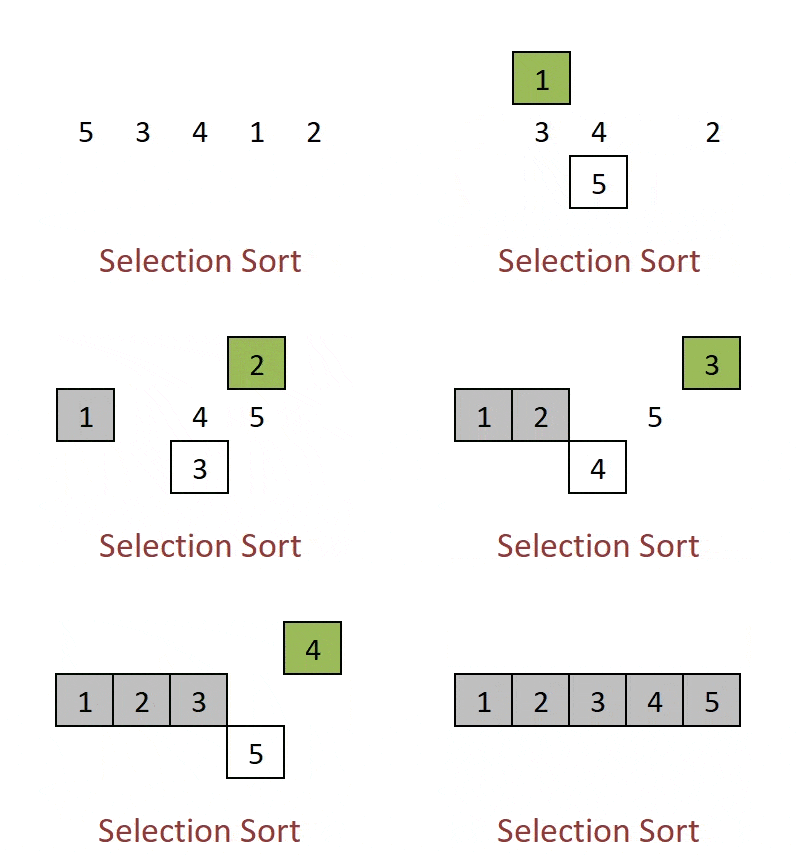
Selection sort builds the sorted portion from the front.
Each pass finds the smallest item in the unsorted portion and swaps it into the next correct position at the front.
How it works:
- Pass 1: Find smallest overall → put it in position 0
- Pass 2: Find smallest in remaining → put it in position 1
- Pass 3: Find smallest in what's left → put it in position 2
- Repeat until all positions filled
Pseudocode:
for i from 0 to length-2:           // position to fill
    minIndex = i                    // assume current is smallest
    for j from i+1 to length-1:     // search remaining unsorted
        if arr[j] < arr[minIndex]:
            minIndex = j           // found smaller
    swap arr[i] with arr[minIndex]  // put smallest in position i
How it works step-by-step:
- Outer loop
i= position we want to fill with correct item - Inner loop searches from
i+1to end for true minimum - Swap minimum into position
i - First
ipositions become permanently sorted after each pass - Last pass only compares 1 item (already sorted)
Key difference from bubble: Finds correct item first, then one swap per pass.
Why it's slow (O(n²))
Selection sort complexity:
| Case | Time | Why |
|---|---|---|
| Best | O(n²) | Still searches entire unsorted portion |
| Average | O(n²) | Always n(n-1)/2 comparisons |
| Worst | O(n²) | Same as average |
Concrete numbers:
- n=100 → ~5,000 comparisons
- n=1,000 → ~500,000 comparisons
- n=10,000 → ~50 million comparisons
Why always O(n²):
Unlike bubble, selection always searches the entire unsorted portion every pass, even if already sorted.
Selection shows "find minimum" pattern. Great for learning, never for real data.
Insertion sort
Insertion sort grows a sorted section one item at a time from left to right.
Each step takes the next unsorted item and slides larger items right until it finds the correct spot.
Tiny example: Sort [6, 3, 8, 2]
How it works:
- Pass 1: First item is sorted `
- Pass 2: Take next item, insert into sorted section
[3, 6] - Pass 3: Take next item, insert into sorted section
[3, 6, 8] - Repeat until all items processed

Pseudocode:
for i from 1 to length-1:           // next item to insert
    key = arr[i]                    // save item to insert
    j = i - 1                       // start from end of sorted part
    while j >= 0 and arr[j] > key:  // shift larger items right
        arr[j+1] = arr[j]
        j = j - 1
    arr[j+1] = key                  // drop key in correct position
How it works step-by-step:
- Outer loop
ipicks next unsorted item (arr[i]) - Save it as
key, startjat end of sorted portion (i-1) - While
arr[j] > keyandj >= 0: shiftarr[j]right toarr[j+1] - Place
keyatarr[j+1](the gap created by shifting) - First
ipositions are sorted after each pass
Key difference from selection: Shifts many items to make space vs one swap.
Why it's slow (O(n²))
Insertion sort complexity:
| Case | Time | Why |
|---|---|---|
| Best (already sorted) | O(n) | No shifting needed |
| Average | O(n²) | ~n²/4 shifts |
| Worst (reverse sorted) | O(n²) | Maximum shifting |
Concrete numbers:
- n=100 → ~2,500 shifts avg
- n=1,000 → ~250,000 shifts
- n=10,000 → ~25 million shifts
Why O(n²): Worst case shifts nearly every item in sorted portion for every new item.
Insertion teaches "build gradually" pattern. Fastest of simple sorts when nearly sorted.
3) Divide and conquer strategies for sorting
Fast sorting algorithms work by breaking big problems into smaller ones.
Instead of comparing every item against every other item, they first split the array into two halves.
Each half gets sorted separately using the same method, then the two sorted halves get combined into one final sorted array.
This "divide → solve → combine" pattern gives O(n log n) speed instead of O(n²).
The same idea powers binary search — check middle, solve half the problem, repeat.
Once you understand this pattern, you'll see it everywhere in algorithms.
Merge sort
Merge sort divides the array in half repeatedly, sorts each half, then merges them back together.
Uses recursion: break into tiny pieces, solve small problems, combine solutions.
How it works:
- Divide array into two halves recursively until single items remain
- Merge pairs of sorted lists by always taking the smaller head
- Repeat until entire array is merged

Pseudocode:
mergeSort(arr, start, end):
    if start < end:                    // more than 1 item
        mid = (start + end) / 2        // split point
        mergeSort(arr, start, mid)     // sort left half
        mergeSort(arr, mid+1, end)     // sort right half
        merge(arr, start, mid, end)    // combine sorted halves

merge(arr, start, mid, end):
    // Compare heads of two sorted halves, take smaller, repeat
How it works step-by-step:
- Recursively split until single elements (base case: 1 item = sorted)
- Merge pairs: compare first items, take smaller, repeat until both empty
- Copy leftovers from either half
- Work doubles back up: 2→4→8→...→n items
Key difference from simple sorts: Uses extra space and recursion instead of swaps.
Why it's fast (O(n log n))
Merge sort complexity:
| Case | Time | Space |
|---|---|---|
| Best | O(n log n) | O(n) |
| Average | O(n log n) | O(n) |
| Worst | O(n log n) | O(n) |
Concrete numbers:
- n=1,000 → ~10,000 comparisons
- n=10,000 → ~140,000 comparisons
- n=1,000,000 → ~20,000,000 comparisons
Why always O(n log n): Always does log n levels of splitting + n work per level.
Merge sort = predictable speed king. Uses extra memory but never fails.
Quick sort
Quick sort picks one number (called the pivot) and rearranges the entire array around it.
After rearranging, the pivot is in its correct final sorted position forever.
Numbers smaller than pivot move to its left. Numbers larger move to its right.
How it works: - Pick pivot (usually last item) - Rearrange: < pivot | pivot | > pivot - Repeat same process on left section AND right section - Pivots stay sorted forever, sections shrink

Pseudocode:
quickSort(arr, low, high):
    if low < high:                      // 2+ items
        pivotIndex = partition(arr, low, high)  // pivot in place
        quickSort(arr, low, pivotIndex-1)       // left side
        quickSort(arr, pivotIndex+1, high)      // right side

partition(arr, low, high):
    pivot = arr[high]                   // choose last as pivot
    i = low - 1                         // boundary for < pivot
    for j from low to high-1:
        if arr[j] <= pivot:
            i = i + 1
            swap arr[i] with arr[j]
    swap arr[i+1] with arr[high]        // put pivot in correct spot
    return i + 1                        // pivot's final position
How it works step-by-step:
partition()rearranges so pivot is in correct final position- All left of pivot < pivot, all right > pivot
- Recurse on left subarray (low to pivotIndex-1)
- Recurse on right subarray (pivotIndex+1 to high)
- Pivot never moves again — permanently sorted
Key difference from merge: Works in-place (no extra space), but average vs worst case varies.
Why it's fast
Quick sort complexity:
| Case | Time | Why |
|---|---|---|
| Best | O(n log n) | Perfect pivot splits |
| Average | O(n log n) | Random pivot works well |
| Worst | O(n²) | Already sorted + bad pivot |
Concrete numbers (average case):
- n=1,000 → ~10,000 operations
- n=10,000 → ~140,000 operations
- n=1,000,000 → ~20,000,000 operations
Why variable speed:
Pivot choice matters. Java uses "dual-pivot" to avoid worst case.
Quick sort = fastest in practice. Java's version is battle-tested and optimized.
Simple sorts summary
All three simple sorts use nested loops and do about n²/2 comparisons.
Bubble swaps adjacent items repeatedly. Selection finds minimum each pass. Insertion builds sorted prefix by shifting.
| Algorithm | How it works | Best case | Swaps | Good for |
|---|---|---|---|---|
| Bubble | Adjacent swaps, bubbles largest right | O(n) already sorted | Many | Learning swaps |
| Selection | Find min → swap to front | Always O(n²) | Few (n swaps) | Learning min-finding |
| Insertion | Shift right → insert in gap | O(n) nearly sorted | Varies | Nearly sorted data |
Key pattern: Outer loop = passes, inner loop = work per pass.
Fast sorts summary
Both break problem into smaller pieces + combine. Merge uses extra space, guaranteed speed. Quick works in-place, usually fast.
| Algorithm | Strategy | Time guarantee | Space | Stable? |
|---|---|---|---|---|
| Merge | Divide → sort → merge | Always O(n log n) | O(n) extra | Yes |
| Quick | Partition around pivot → recurse | Average O(n log n), worst O(n²) | O(log n) | No |
Production rule: Use Java built-ins (both use optimized Quick/Merge hybrids).
Simple sorts teach you how. Fast sorts teach you why. Java built-ins teach you what to actually use.